


Structural Learning for Continuous Data -- A Benchmark of State-of-the-Art Algorithms
Benchmarking structure-learning algorithms for continuous data
Modeling a high-dimensional multivariate distribution is hard. In the discrete case, Bayesian networks are a well-established way to cut down the complexity by factorizing the joint distribution into a product of local conditional distributions. The continuous case is messier: there is no single general-purpose model, and over the past three decades the community has produced a wide range of structure-learning algorithms — constraint-based, score-based, and continuous-optimization methods. The problem is that each of them makes different assumptions about the data (linearity, noise distribution, …), and those assumptions largely decide whether a method works well or poorly.
This post summarizes a benchmark of several state-of-the-art algorithms across a range of continuous datasets. We compare them with structural metrics and try to answer a practical question: when does each method do well, when does it break, and is there a reasonable default? The short version is that no algorithm dominates everywhere, and copula-based methods are the most consistent.
The algorithms
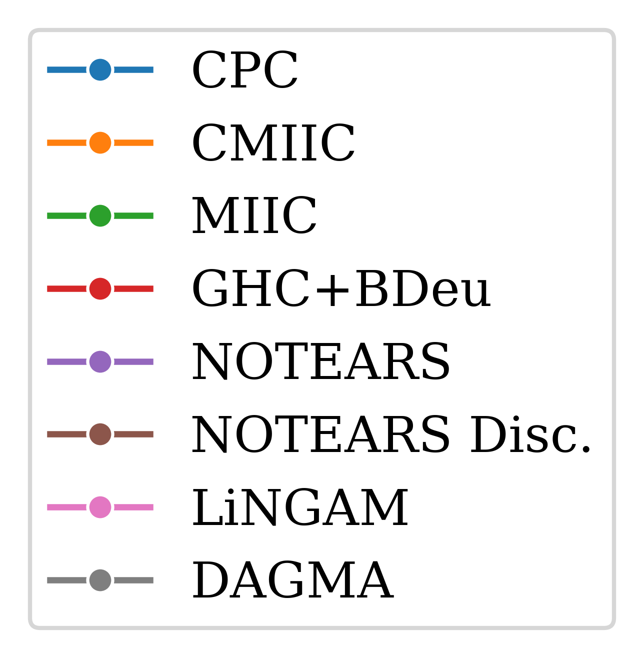
We compare eight algorithms, spanning three families:
- Constraint-based / information-theoretic: ContinuousPC and ContinuousMIIC (both copula-based, from otagrum), and MIIC.
- Score-based: GHC+BDeu (greedy hill climbing with a BDeu score).
- Continuous-optimization: NOTEARS, DAGMA, and DirectLiNGAM.
ContinuousPC, ContinuousMIIC, NOTEARS and DirectLiNGAM work on continuous data natively; MIIC and GHC+BDeu need a discretization step first. We also include a Discrete NOTEARS variant — NOTEARS applied to discretized data.
Because observational data only identifies a graph up to its Markov equivalence class, every algorithm outputs a completed partially directed acyclic graph (a CPDAG), and we evaluate against that.
How the benchmark works
Data. We use one real and five synthetic settings:
- An experimental dataset: the Sachs protein-signaling data (853 measurements), evaluated against a biologically-curated 18-edge ground truth.
- Five synthetic regimes chosen to stress different assumptions: linear SEMs with Gaussian and Laplace noise, and Copula Bayesian Networks with Gaussian, Clayton, and Gaussian-mixture copulas.
Protocol. For the synthetic data, we generate 30 random graphs per setting, at 20 variables, and increase the number of samples from 200 to 5000. This shows not only who wins, but how each method behaves as data grows. Hyperparameters are selected per algorithm by grid search against the ground truth.
Metrics. In this post we focus on two complementary metrics, both computed on the CPDAG:
- SHD (Structural Hamming Distance): edge edits needed to match the truth — lower is better;
- F1-score: harmonic mean of precision and recall — higher is better;
The figures below all report metrics on CPDAGs for the 20-variable case.
Results on the experimental dataset
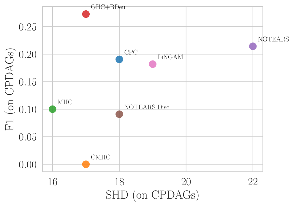
Sachs Data |
On Sachs, scores are low across the board — both because of the difficulty of the problem and because the ground truth is sparse, which makes it easier to add a wrong edge than to find a right one. The points are scattered along a diagonal: a method tends to have either a good SHD or a good F1, but not both, which already tells us the two metrics do not carry the same information. GHC+BDeu and MIIC sit on the Pareto front; both learn few edges, but a good fraction of them are correct. NOTEARS learns many edges, most of them wrong (high SHD). ContinuousMIIC ends up at an F1 of 0 on the CPDAGs because it does not orient any of the few edges it finds.
DAGMA is missing from the plot: on the raw Sachs measurements its least-squares objective is not scale-invariant, and with standard deviations ranging from ~10 to ~430 across proteins it systematically fails to return a valid DAG (it works again on the log-transformed data). This scale-sensitivity is a known evaluation bias of NOTEARS-family methods.
Results on the synthetic datasets
CBN — Uniform marginals / Gaussian copulas
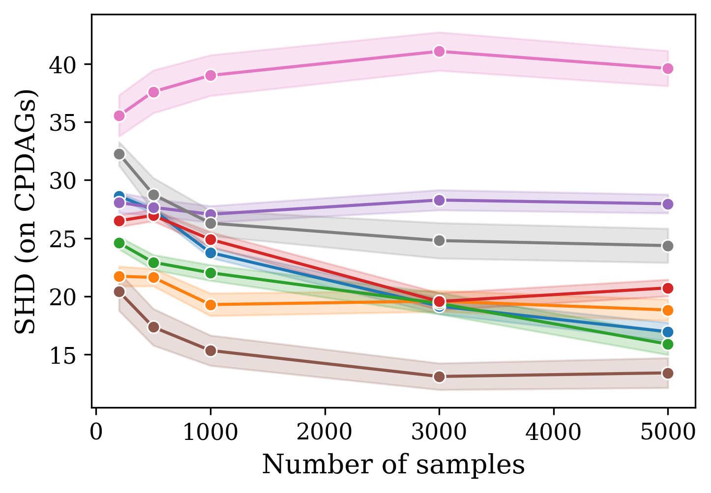
Gaussian copula |
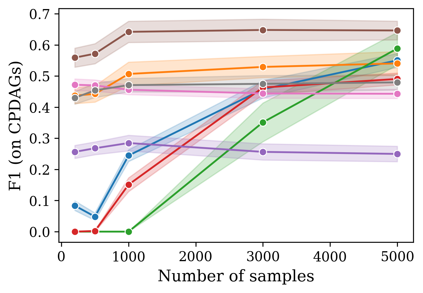
|
Most methods do reasonably well here and improve with more samples. Discrete NOTEARS is the strongest, though it fails to return a valid DAG about one run in three (see the error-rate analysis below). LiNGAM recovers many edges, but also many wrong ones, which inflates its SHD. ContinuousPC is weak at small sample sizes — small sample size independence tests introduce errors that then propagate.
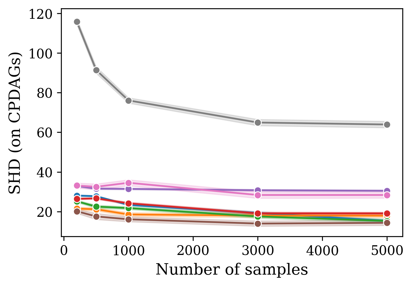
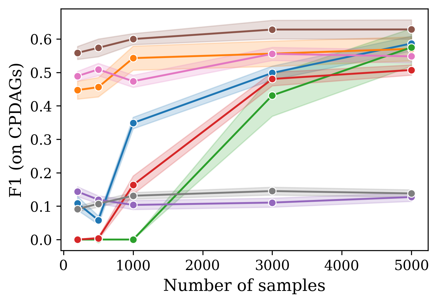
CBN — Exponential marginals / Clayton copulas
Clayton copulas |
|
The non-linear dependencies hurt NOTEARS and DAGMA badly — neither is designed for them. Discrete NOTEARS and ContinuousMIIC clearly outperform the others on this dataset. DAGMA creates many more edges than NOTEARS, which raises its SHD, and LiNGAM again learns too many edges, many of them spurious.
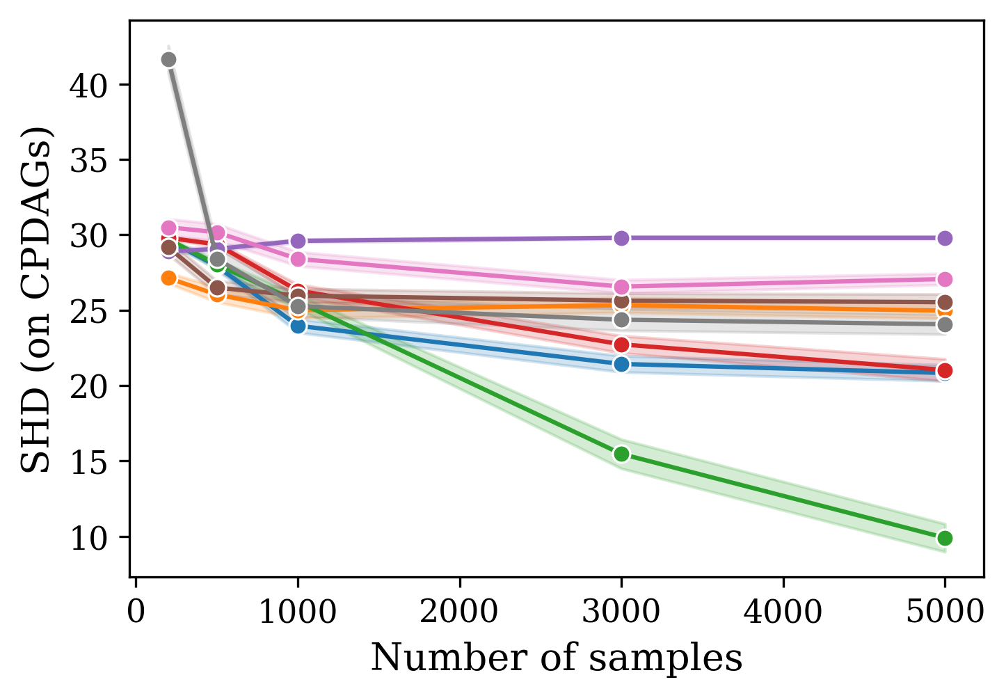
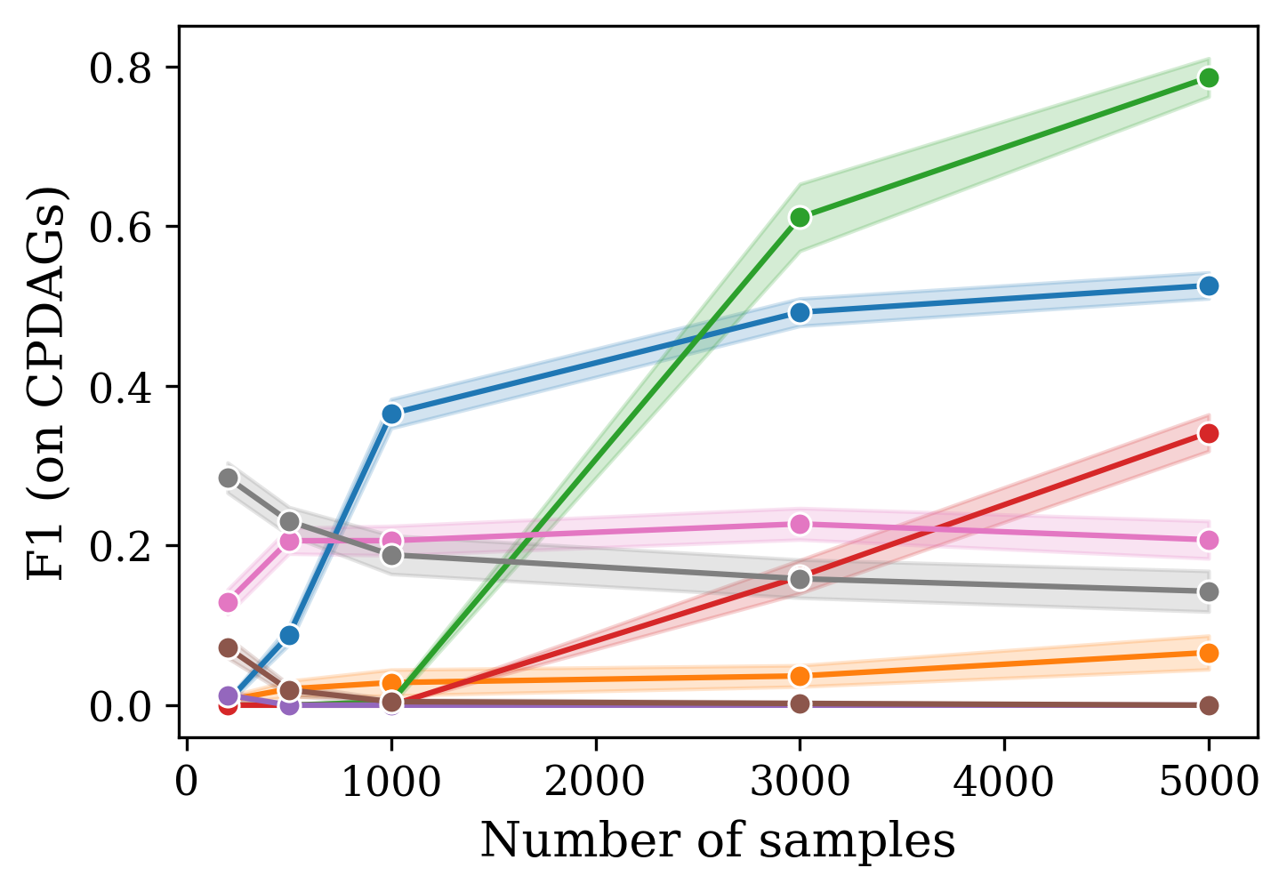
CBN — Uniform marginals / Gaussian-mixture copulas
Gaussian-mixture copulas |
|
This is a hard dataset where almost every method struggles. Discretized MIIC and ContinuousPC cope best, taking advantage of the larger sample sizes. Interestingly, discretized MIIC beats ContinuousMIIC here, which suggests that for this regime discretization captures the dependencies better than the Empirical Bernstein Copula estimator.
Linear SEM — Gaussian noise
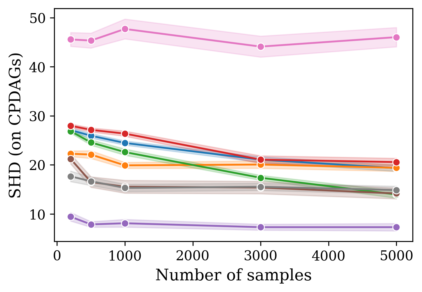
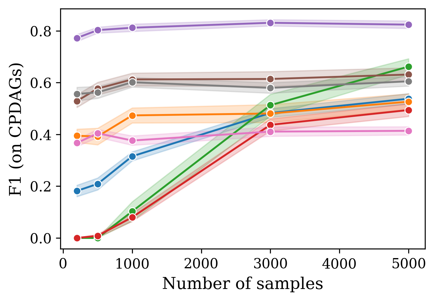
Linear SEM - Gaussian noise |
|
NOTEARS is built for exactly this linear-Gaussian setting, and it performs best here. LiNGAM does poorly — it relies on non-Gaussian noise to orient edges, which it does not have here. Discretizing hurts NOTEARS (information loss), and DAGMA trails NOTEARS.
Linear SEM — Laplace noise
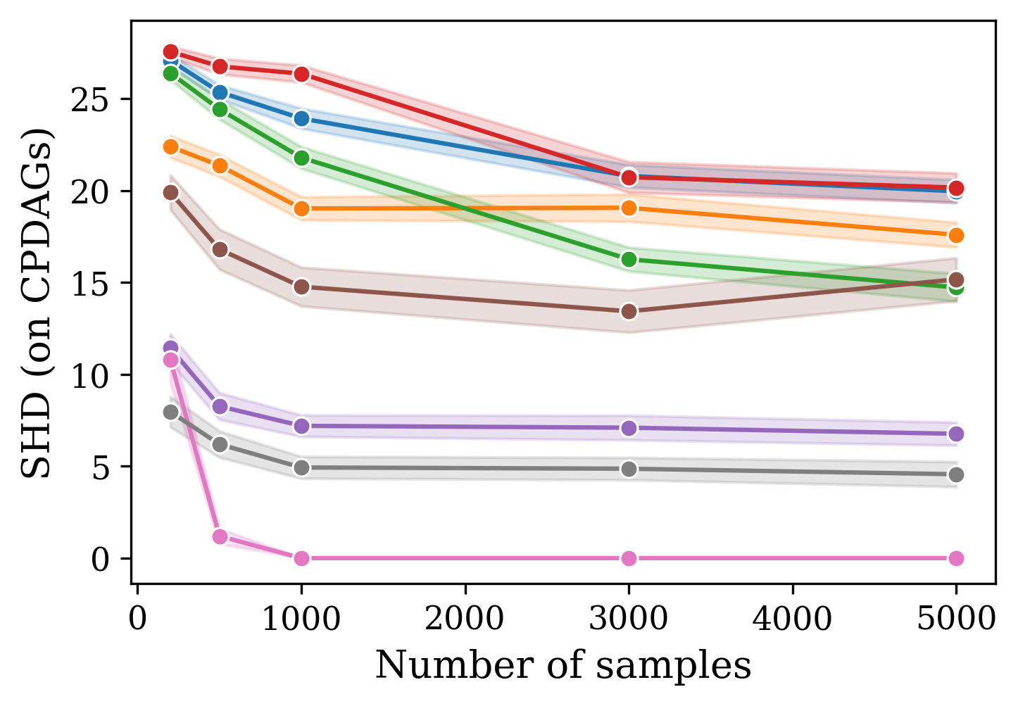
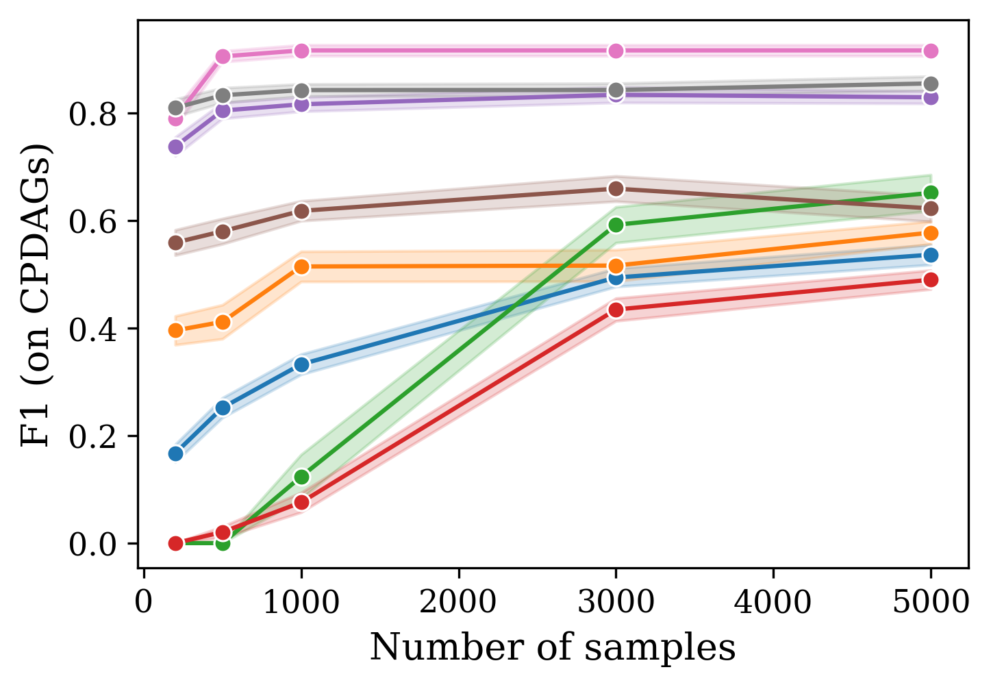
Linear SEM - Laplace noise |
|
The model is still linear, but the noise is now non-Gaussian — which lets LiNGAM overtake NOTEARS, since non-Gaussianity is exactly what it exploits to orient edges. The optimization-based trio (NOTEARS, DAGMA, LiNGAM) leads, and the other methods follow closely.
When do algorithms fail to return a DAG?

Sachs Data |
Some methods can fail to produce a valid DAG, in which case the run is dropped. ContinuousPC, ContinuousMIIC, MIIC and GHC+BDeu are guaranteed to return a DAG and never appear here. Among the rest, Discrete NOTEARS is by far the least reliable, failing much more often than NOTEARS. DAGMA struggles on the small-sample Clayton data, and NOTEARS fails most at 20 variables — ironically on the Gaussian-copula and Clayton datasets, which are otherwise among its better cases.
Discussion and conclusion
No algorithm dominates across all datasets: each method has a regime in which it excels and another in which it fails. Continuous-optimization methods (NOTEARS, DAGMA) perform best on linear SEMs but degrade sharply on non-linear copula-based data; LiNGAM shines when the noise is clearly non-Gaussian but produces many spurious edges otherwise; constraint-based and information-theoretic methods (ContinuousPC, ContinuousMIIC, MIIC) are the most consistent across regimes, at the cost of weaker peak performance on their favorable cases. Discretization, often treated as a naive preprocessing step, turns out to be surprisingly effective, and copula-based methods stand out for their stable behavior when the data-generating distribution is unknown.
To compress this into a single view, we rank the algorithms on each dataset (using successive Pareto fronts on SHD/F1, refined by F1), then average those ranks over the five synthetic regimes at 5000 samples:
| Algorithm | Average rank |
|---|---|
| ContinuousPC | 3.1 |
| MIIC | 3.3 |
| Discrete NOTEARS | 3.7 |
| DirectLiNGAM | 4.1 |
| DAGMA | 4.8 |
| NOTEARS | 5.5 |
| ContinuousMIIC | 5.6 |
| GHC+BDeu | 5.9 |
ContinuousPC comes out ahead of ContinuousMIIC because we rank at 5000 samples — precisely where ContinuousPC overtakes it. On smaller datasets the picture reverses: ContinuousMIIC starts very strong but then plateaus as the sample size grows, while ContinuousPC keeps improving. The likely reason is that ContinuousMIIC’s independence test uses a fixed threshold that does not depend on the sample size, which helps when data is scarce but limits it when it is bigger.
The main takeaways:
- No algorithm is uniformly strong. On realistic continuous data, state-of-the-art methods reach only moderate accuracy, and their relative ranking depends heavily on the data distribution.
- Copula-based methods are the most consistent across distributional regimes, which makes them an attractive default when the data-generating distribution is unknown.
- Discretization is less naive than it looks. Despite the information loss, several discretization-based methods are very competitive, and Discrete NOTEARS even beats its continuous counterpart on some datasets.
- MIIC performs consistently well, supporting the relevance of information-theoretic approaches.
- Evaluation metrics remain a bottleneck. SHD and F1 capture complementary but partial aspects of graph quality and can produce contradictory rankings.