Approximate inference in aGrUM (pyAgrum)

There are several approximate inference for BN in aGrUM (pyAgrum). They share the same API than exact inference.

• Loopy Belief Propagation : LBP is an approximate inference that uses exact calculous methods (when the BN os a tree) even if the BN is not a tree. LBP is a special case of inference : the algorithm may not converge and even if it converges, it may converge to anything (but the exact posterior). LBP however is fast and usually gives not so bad results.
• Sampling inference : Sampling inference use sampling to compute the posterior. The sampling may be (very) slow but those algorithms converge to the exac distribution. aGrUM implements :
  • Montecarlo sampling,
  • Weighted sampling,
  • Importance sampling,
  • Gibbs sampling.
• Finally, aGrUM propose the so-called ‘loopy version’ of the sampling algorithms : the idea is to use LBP as a Dirichlet prior for the sampling algorithm. A loopy version of each sampling algorithm is proposed.

%matplotlib inline
from pylab import *
import matplotlib.pyplot as plt


def unsharpen(bn):
  """
  Force the parameters of the BN not to be a bit more far from 0 or 1
  """
  for nod in bn.nodes():
    bn.cpt(nod).translate(bn.maxParam() / 10).normalizeAsCPT()


def compareInference(ie, ie2, ax=None):
  """
  compare 2 inference by plotting all the points from (posterior(ie),posterior(ie2))
  """
  exact = []
  appro = []
  errmax = 0
  for node in bn.nodes():
    # Tensors as list
    exact += ie.posterior(node).tolist()
    appro += ie2.posterior(node).tolist()
    errmax = max(errmax, (ie.posterior(node) - ie2.posterior(node)).abs().max())

  if errmax < 1e-10:
    errmax = 0
  if ax == None:
    fig = plt.Figure(figsize=(4, 4))
    ax = plt.gca()  # default axis for plt

  ax.plot(exact, appro, "ro")
  ax.set_title(
    "{} vs {}\n {}\nMax error {:2.4} in {:2.4} seconds".format(
      str(type(ie)).split(".")[2].split("_")[0][0:-2],  # name of first inference
      str(type(ie2)).split(".")[2].split("_")[0][0:-2],  # name of second inference
      ie2.messageApproximationScheme(),
      errmax,
      ie2.currentTime(),
    )
  )

import pyagrum as gum
import pyagrum.lib.notebook as gnb

bn = gum.loadBN("res/alarm.bgum")
unsharpen(bn)

ie = gum.LazyPropagation(bn)
ie.makeInference()

gnb.showBN(bn, size="8")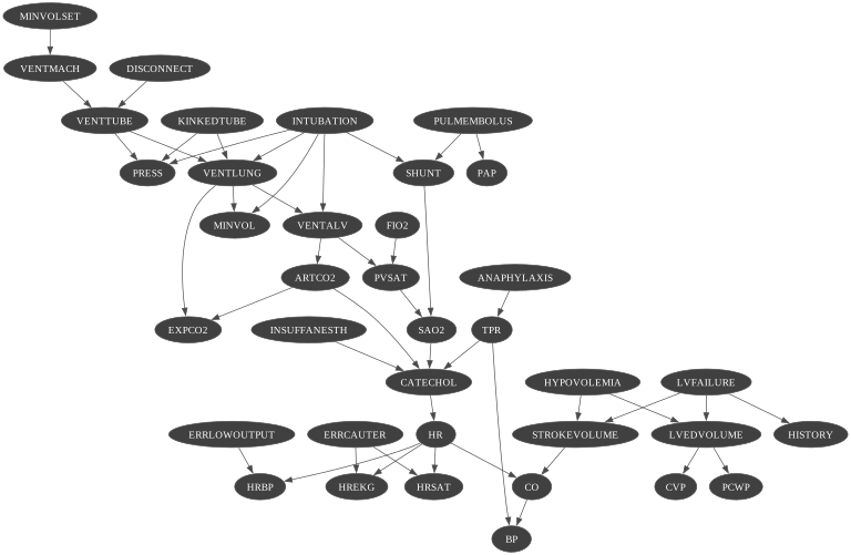

First, an exact inference.

gnb.sideBySide(gnb.getJunctionTreeMap(bn), gnb.getInference(bn, size="8"))  # using LazyPropagation by default
print(ie.posterior("KINKEDTUBE"))

  KINKEDTUBE       │
TRUE     │FALSE    │
─────────│─────────│
 0.1167  │ 0.8833  │

Gibbs Inference

Gibbs inference with default parameters

Gibbs inference iterations can be stopped :

• by the value of error (epsilon)
• by the rate of change of epsilon (MinEpsilonRate)
• by the number of iteration (MaxIteration)
• by the duration of the algorithm (MaxTime)

ie2 = gum.GibbsSampling(bn)
ie2.setEpsilon(1e-2)
gnb.showInference(bn, engine=ie2, size="8")
print(ie2.posterior("KINKEDTUBE"))
print(ie2.messageApproximationScheme())
compareInference(ie, ie2)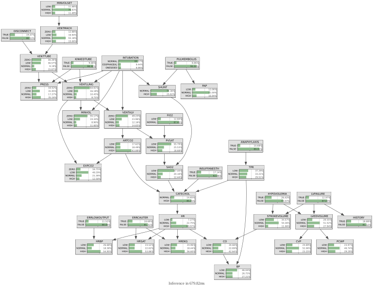

  KINKEDTUBE       │
TRUE     │FALSE    │
─────────│─────────│
 0.1068  │ 0.8932  │

stopped with rate=0.006737946999085467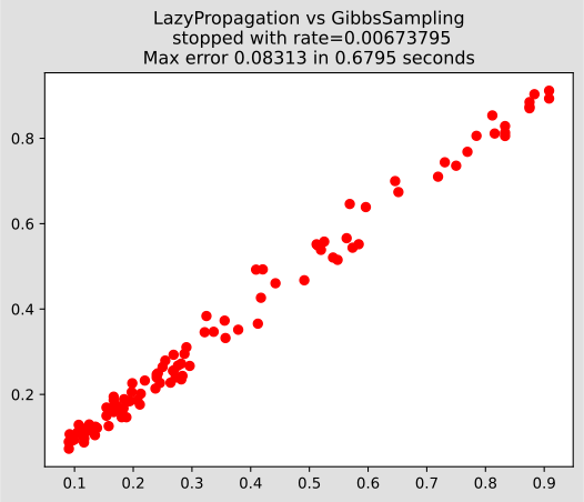

With default parameters, this inference has been stopped by a low value of rate.

Changing parameters

ie2 = gum.GibbsSampling(bn)
ie2.setMaxIter(1000)
ie2.setEpsilon(5e-3)
ie2.makeInference()

print(ie2.posterior(2))
print(ie2.messageApproximationScheme())

  INTUBATION                 │
NORMAL   │ESOPHAGEA│ONESIDED │
─────────│─────────│─────────│
 0.6870  │ 0.1910  │ 0.1220  │

stopped with max iteration=1000

compareInference(ie, ie2)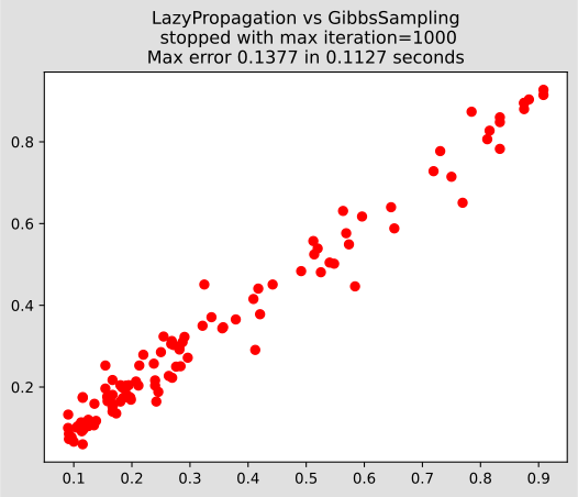

ie2 = gum.GibbsSampling(bn)
ie2.setMaxTime(3)
ie2.makeInference()

print(ie2.posterior(2))
print(ie2.messageApproximationScheme())
compareInference(ie, ie2)

  INTUBATION                 │
NORMAL   │ESOPHAGEA│ONESIDED │
─────────│─────────│─────────│
 0.8000  │ 0.1967  │ 0.0033  │

stopped with epsilon=0.20189651799465538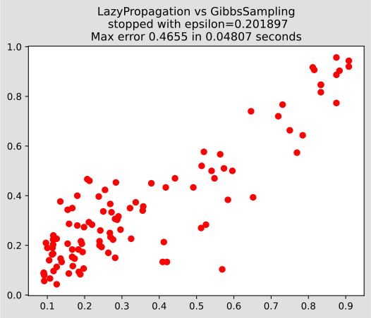

Looking at the convergence

ie2 = gum.GibbsSampling(bn)
ie2.setEpsilon(10**-1.8)
ie2.setBurnIn(300)
ie2.setPeriodSize(300)
ie2.setDrawnAtRandom(True)
gnb.animApproximationScheme(ie2)
ie2.makeInference()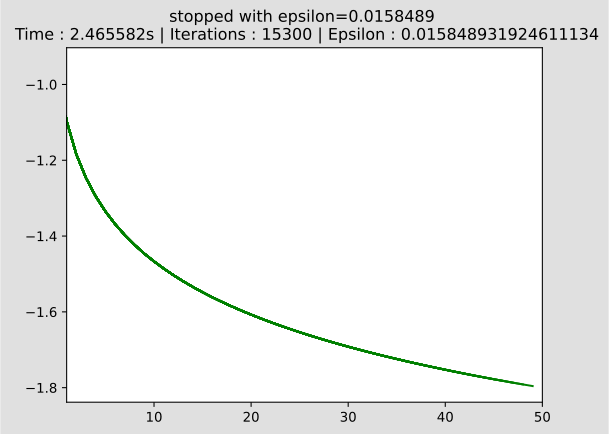

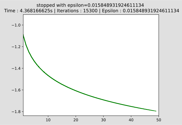
compareInference(ie, ie2)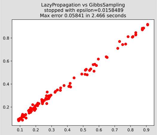

Importance Sampling

ie4 = gum.ImportanceSampling(bn)
ie4.setEpsilon(10**-1.8)
ie4.setMaxTime(10)  # 10 seconds for inference
ie4.setPeriodSize(300)
ie4.makeInference()
compareInference(ie, ie4)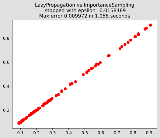

Loopy Gibbs Sampling

Every sampling inference has a ‘hybrid’ version which consists in using a first loopy belief inference as a prior for the probability estimations by sampling.

ie3 = gum.LoopyGibbsSampling(bn)

ie3.setEpsilon(10**-1.8)
ie3.setMaxTime(10)  # 10 seconds for inference
ie3.setPeriodSize(300)
ie3.makeInference()
compareInference(ie, ie3)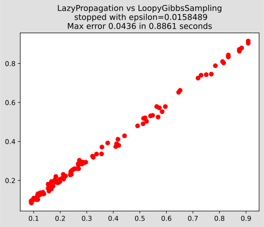

Comparison of approximate inference

These computations may be a bit long

def compareAllInference(bn, evs={}, epsilon=10**-1.6, epsilonRate=1e-8, maxTime=20):
  ies = [
    gum.LazyPropagation(bn),
    gum.LoopyBeliefPropagation(bn),
    gum.GibbsSampling(bn),
    gum.LoopyGibbsSampling(bn),
    gum.WeightedSampling(bn),
    gum.LoopyWeightedSampling(bn),
    gum.ImportanceSampling(bn),
    gum.LoopyImportanceSampling(bn),
  ]

  # burn in for Gibbs samplings
  for i in [2, 3]:
    ies[i].setBurnIn(300)
    ies[i].setDrawnAtRandom(True)

  for i in range(2, len(ies)):
    ies[i].setEpsilon(epsilon)
    ies[i].setMinEpsilonRate(epsilonRate)
    ies[i].setPeriodSize(300)
    ies[i].setMaxTime(maxTime)

  for i in range(len(ies)):
    ies[i].setEvidence(evs)
    ies[i].makeInference()

  fig, axes = plt.subplots(1, len(ies) - 1, figsize=(35, 3), num="gpplot")
  for i in range(len(ies) - 1):
    compareInference(ies[0], ies[i + 1], axes[i])

Inference stopped by epsilon

compareAllInference(bn, epsilon=1e-1)

compareAllInference(bn, epsilon=1e-2)

inference stopped by time

compareAllInference(bn, maxTime=1, epsilon=1e-8)

compareAllInference(bn, maxTime=2, epsilon=1e-8)

Inference with Evidence (more complex)

funny = {"BP": 1, "PCWP": 2, "EXPCO2": 0, "HISTORY": 0}
compareAllInference(bn, maxTime=1, evs=funny, epsilon=1e-8)

compareAllInference(bn, maxTime=4, evs=funny, epsilon=1e-8)

compareAllInference(bn, maxTime=10, evs=funny, epsilon=1e-8)