Skip to content

Probablistic Inference with pyAgrum

Creative Commons LicenseaGrUMinteractive online version

In this notebook, we will show different basic features for probabilistic inference on Bayesian networks using pyagrum.

First we need some external modules:

Then we import pyagrum and the pyAgrum’s notebook module, that offers very usefull methods when writting a notebook.

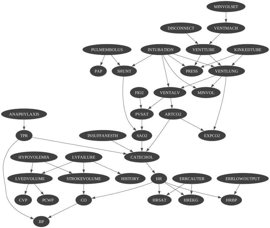
This first example shows how you can load a BayesNet and show it as graph. Note that pyAgrum handles serveral BayesNet file format such as DSL, BIF and UAI.

import pyagrum as gum
import pyagrum.lib.notebook as gnb
bn = gum.loadBN("res/alarm.bgum")
gnb.showBN(bn, size="9")

svg

print(bn)
BN{nodes: 37, arcs: 46, domainSize: 10^16.2389, dim: 509, mem: 5Ko 896o}

From there, it is easy to get a posterior using an inference engine :

ie = gum.LazyPropagation(bn)
ie.makeInference()
print(ie.posterior(bn.idFromName("CATECHOL")))
CATECHOL │
NORMAL │HIGH │
─────────│─────────│
0.0512 │ 0.9488 │

But since we are in notebook, why not use pyAgrum notebook’s methods ?

gnb.showPosterior(bn, evs={}, target="CATECHOL")
PyAgrum inline image

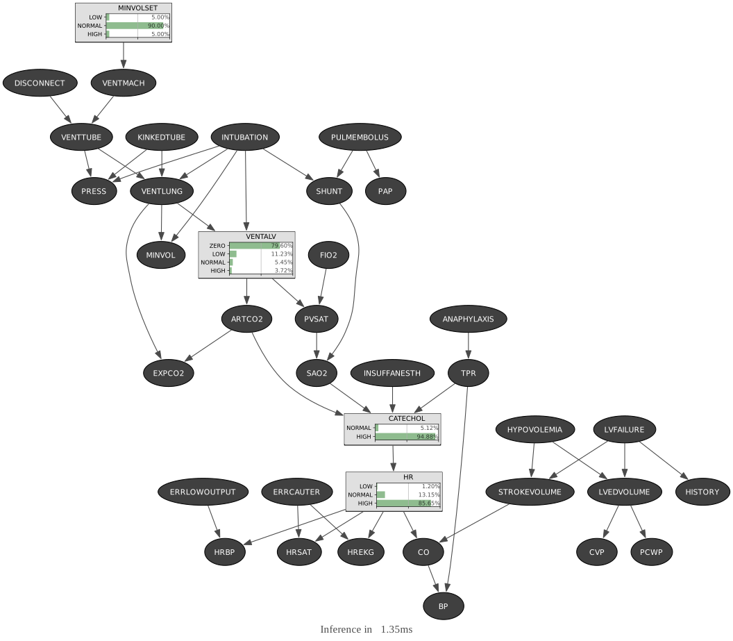
You may also want to see the graph with some posteriors

## due to matplotlib, format is forced to png.
gnb.showInference(bn, evs={}, targets={"VENTALV", "CATECHOL", "HR", "MINVOLSET"}, size="11")
svg

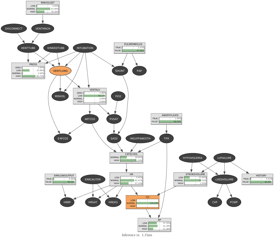
.. and then observe the impact of evidence :

gnb.showInference(
bn,
evs={"CO": 1, "VENTLUNG": 1},
targets={
"VENTALV",
"CATECHOL",
"HR",
"MINVOLSET",
"ANAPHYLAXIS",
"STROKEVOLUME",
"ERRLOWOUTPUT",
"HBR",
"PULMEMBOLUS",
"HISTORY",
"BP",
"PRESS",
"CO",
},
size="10",
)

svg

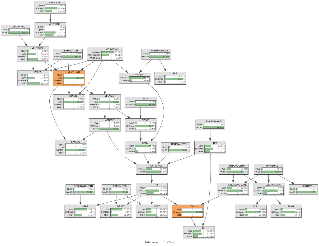
You can even compute all posteriors by leaving the targets parameter empty (which is its default value).

gnb.showInference(bn, evs={"CO": 1, "VENTLUNG": 1}, size="14")
svg

To have a global view of the knowledge brought by the inference, you can also draw the entropy of all nodes

import pyagrum.explain as explain
explain.showInformation(bn, {}, size="14")
G CVP CVP SHUNT SHUNT SAO2 SAO2 SHUNT->SAO2 ANAPHYLAXIS ANAPHYLAXIS TPR TPR ANAPHYLAXIS->TPR MINVOL MINVOL LVEDVOLUME LVEDVOLUME LVEDVOLUME->CVP PCWP PCWP LVEDVOLUME->PCWP KINKEDTUBE KINKEDTUBE PRESS PRESS KINKEDTUBE->PRESS VENTLUNG VENTLUNG KINKEDTUBE->VENTLUNG FIO2 FIO2 PVSAT PVSAT FIO2->PVSAT BP BP HYPOVOLEMIA HYPOVOLEMIA HYPOVOLEMIA->LVEDVOLUME STROKEVOLUME STROKEVOLUME HYPOVOLEMIA->STROKEVOLUME ERRCAUTER ERRCAUTER HREKG HREKG ERRCAUTER->HREKG HRSAT HRSAT ERRCAUTER->HRSAT INSUFFANESTH INSUFFANESTH CATECHOL CATECHOL INSUFFANESTH->CATECHOL HR HR HR->HREKG CO CO HR->CO HR->HRSAT HRBP HRBP HR->HRBP CO->BP CATECHOL->HR SAO2->CATECHOL INTUBATION INTUBATION INTUBATION->SHUNT INTUBATION->MINVOL INTUBATION->PRESS INTUBATION->VENTLUNG VENTALV VENTALV INTUBATION->VENTALV DISCONNECT DISCONNECT VENTTUBE VENTTUBE DISCONNECT->VENTTUBE PAP PAP PVSAT->SAO2 LVFAILURE LVFAILURE LVFAILURE->LVEDVOLUME LVFAILURE->STROKEVOLUME HISTORY HISTORY LVFAILURE->HISTORY TPR->BP TPR->CATECHOL ERRLOWOUTPUT ERRLOWOUTPUT ERRLOWOUTPUT->HRBP EXPCO2 EXPCO2 MINVOLSET MINVOLSET VENTMACH VENTMACH MINVOLSET->VENTMACH VENTTUBE->PRESS VENTTUBE->VENTLUNG STROKEVOLUME->CO VENTLUNG->MINVOL VENTLUNG->EXPCO2 VENTLUNG->VENTALV VENTMACH->VENTTUBE VENTALV->PVSAT ARTCO2 ARTCO2 VENTALV->ARTCO2 ARTCO2->CATECHOL ARTCO2->EXPCO2 PULMEMBOLUS PULMEMBOLUS PULMEMBOLUS->SHUNT PULMEMBOLUS->PAP
PyAgrum inline image

… and then observe the impact of an evidence on the whole bayes network :

explain.showInformation(bn, {"CO": 0}, size="9")
G CVP CVP SHUNT SHUNT SAO2 SAO2 SHUNT->SAO2 ANAPHYLAXIS ANAPHYLAXIS TPR TPR ANAPHYLAXIS->TPR MINVOL MINVOL LVEDVOLUME LVEDVOLUME LVEDVOLUME->CVP PCWP PCWP LVEDVOLUME->PCWP KINKEDTUBE KINKEDTUBE PRESS PRESS KINKEDTUBE->PRESS VENTLUNG VENTLUNG KINKEDTUBE->VENTLUNG FIO2 FIO2 PVSAT PVSAT FIO2->PVSAT BP BP HYPOVOLEMIA HYPOVOLEMIA HYPOVOLEMIA->LVEDVOLUME STROKEVOLUME STROKEVOLUME HYPOVOLEMIA->STROKEVOLUME ERRCAUTER ERRCAUTER HREKG HREKG ERRCAUTER->HREKG HRSAT HRSAT ERRCAUTER->HRSAT INSUFFANESTH INSUFFANESTH CATECHOL CATECHOL INSUFFANESTH->CATECHOL HR HR HR->HREKG CO CO HR->CO HR->HRSAT HRBP HRBP HR->HRBP CO->BP CATECHOL->HR SAO2->CATECHOL INTUBATION INTUBATION INTUBATION->SHUNT INTUBATION->MINVOL INTUBATION->PRESS INTUBATION->VENTLUNG VENTALV VENTALV INTUBATION->VENTALV DISCONNECT DISCONNECT VENTTUBE VENTTUBE DISCONNECT->VENTTUBE PAP PAP PVSAT->SAO2 LVFAILURE LVFAILURE LVFAILURE->LVEDVOLUME LVFAILURE->STROKEVOLUME HISTORY HISTORY LVFAILURE->HISTORY TPR->BP TPR->CATECHOL ERRLOWOUTPUT ERRLOWOUTPUT ERRLOWOUTPUT->HRBP EXPCO2 EXPCO2 MINVOLSET MINVOLSET VENTMACH VENTMACH MINVOLSET->VENTMACH VENTTUBE->PRESS VENTTUBE->VENTLUNG STROKEVOLUME->CO VENTLUNG->MINVOL VENTLUNG->EXPCO2 VENTLUNG->VENTALV VENTMACH->VENTTUBE VENTALV->PVSAT ARTCO2 ARTCO2 VENTALV->ARTCO2 ARTCO2->CATECHOL ARTCO2->EXPCO2 PULMEMBOLUS PULMEMBOLUS PULMEMBOLUS->SHUNT PULMEMBOLUS->PAP
PyAgrum inline image

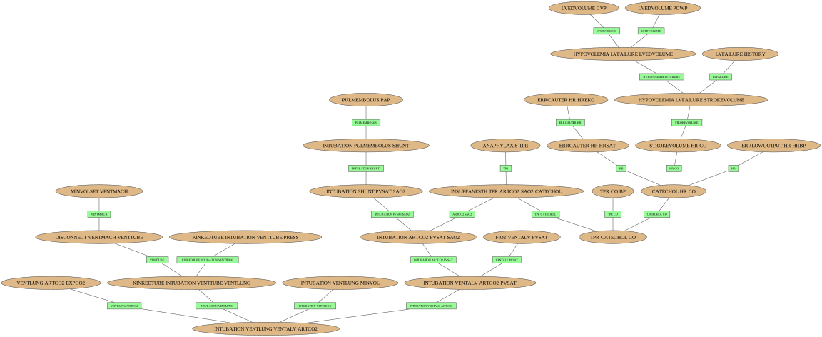
Lazy Propagation, like several other inference algorithms, uses a junction tree to propagate information.

You can show the junction tree used by Lazy Propagation with pyAgrum:

jt = ie.junctionTree()
gnb.showJunctionTree(bn, size="12")

svg

## another representation of the junction, more convenient for investigating the flow of data in the jt
## the size/width of cliques and separators are proportionnal to the number of nodes in the factor.
jt.map()
0 0~16 0--0~16 1 1~32 1--1~32 2 2~33 2--2~33 3 3~4 3--3~4 4 4~22 4--4~22 5 5~22 5--5~22 6 6~23 6--6~23 7 7~26 7--7~26 8 8~17 8--8~17 10 10~14 10--10~14 11 11~16 11--11~16 12 12~13 12--12~13 13 13~30 13--13~30 14 14~26 14--14~26 16 16~17 16--16~17 17 17~24 17--17~24 19 19~27 19--19~27 20 20~33 20--20~33 22 22~33 22--22~33 23 23~27 23--23~27 23~31 23--23~31 24 24~26 24--24~26 26 26~27 26--26~27 27 30 30~31 30--30~31 31 31~32 31--31~32 32 32~33 32--32~33 33 19~27--27 12~13--13 2~33--33 23~27--27 22~33--33 11~16--16 24~26--26 31~32--32 10~14--14 26~27--27 13~30--30 5~22--22 7~26--26 20~33--33 16~17--17 32~33--33 23~31--31 8~17--17 1~32--32 3~4--4 4~22--22 17~24--24 14~26--26 30~31--31 6~23--23 0~16--16

One can easily walk through the junction tree.

for n in jt.nodes():
print([bn.variable(n).name() for n in jt.clique(n)])
['CVP', 'LVEDVOLUME']
['FIO2', 'VENTALV', 'PVSAT']
['ARTCO2', 'EXPCO2', 'VENTLUNG']
['VENTMACH', 'MINVOLSET']
['VENTMACH', 'DISCONNECT', 'VENTTUBE']
['PRESS', 'KINKEDTUBE', 'INTUBATION', 'VENTTUBE']
['ANAPHYLAXIS', 'TPR']
['HRBP', 'ERRLOWOUTPUT', 'HR']
['LVFAILURE', 'HISTORY']
['HREKG', 'HR', 'ERRCAUTER']
['PCWP', 'LVEDVOLUME']
['PAP', 'PULMEMBOLUS']
['SHUNT', 'INTUBATION', 'PULMEMBOLUS']
['HRSAT', 'HR', 'ERRCAUTER']
['LVFAILURE', 'HYPOVOLEMIA', 'LVEDVOLUME']
['HYPOVOLEMIA', 'STROKEVOLUME', 'LVFAILURE']
['CO', 'BP', 'TPR']
['INTUBATION', 'VENTLUNG', 'MINVOL']
['KINKEDTUBE', 'INTUBATION', 'VENTTUBE', 'VENTLUNG']
['INSUFFANESTH', 'TPR', 'ARTCO2', 'SAO2', 'CATECHOL']
['CO', 'STROKEVOLUME', 'HR']
['CO', 'CATECHOL', 'HR']
['CO', 'TPR', 'CATECHOL']
['INTUBATION', 'SHUNT', 'PVSAT', 'SAO2']
['INTUBATION', 'ARTCO2', 'PVSAT', 'SAO2']
['ARTCO2', 'VENTALV', 'INTUBATION', 'PVSAT']
['VENTALV', 'INTUBATION', 'ARTCO2', 'VENTLUNG']
for e in jt.edges():
print(f"Separator for {e} : {jt.clique(e[0]).intersection(jt.clique(e[1]))}")
Separator for (13, 30) : {18, 2}
Separator for (2, 33) : {26, 22}
Separator for (3, 4) : {16}
Separator for (26, 27) : {34, 30}
Separator for (7, 26) : {31}
Separator for (12, 13) : {4}
Separator for (31, 32) : {27, 26, 2}
Separator for (23, 31) : {26, 28}
Separator for (5, 22) : {0, 2, 20}
Separator for (17, 24) : {13}
Separator for (19, 27) : {34, 14}
Separator for (24, 26) : {34, 31}
Separator for (32, 33) : {25, 2, 26}
Separator for (6, 23) : {14}
Separator for (23, 27) : {14, 30}
Separator for (11, 16) : {15}
Separator for (10, 14) : {7, 31}
Separator for (8, 17) : {9}
Separator for (0, 16) : {15}
Separator for (1, 32) : {25, 27}
Separator for (20, 33) : {2, 22}
Separator for (4, 22) : {20}
Separator for (14, 26) : {31}
Separator for (22, 33) : {2, 22}
Separator for (30, 31) : {2, 27, 28}
Separator for (16, 17) : {1, 9}
jt.hasRunningIntersection()
True

The junction tree created by a LazyPropagation is optimized for the query (see RelevanceReasonning notebook). But you can also introspect a junction tree directly from a BN or a graph using the JunctionTreeGenerator’s class.

bn = gum.fastBN("0->1->2<-3->4->5->6<-2->7")
jtg = gum.JunctionTreeGenerator()
gnb.sideBySide(
bn,
jtg.junctionTree(bn),
jtg.eliminationOrder(bn),
jtg.binaryJoinTree(bn),
captions=[
"A Bayesien network",
"a junction tree for this BN",
"its elimination order",
"an (optimized) binary join tree",
],
)
G 1 1 2 2 1->2 7 7 2->7 6 6 2->6 0 0 0->1 3 3 3->2 4 4 3->4 5 5 4->5 5->6
A Bayesien network
(0) 2-5-6 2-5-6 (0) 2-5-6^(4) 2-3-5 2-5 (0) 2-5-6--(0) 2-5-6^(4) 2-3-5 (1) 2-7 2-7 (1) 2-7^(4) 2-3-5 2 (1) 2-7--(1) 2-7^(4) 2-3-5 (2) 0-1 0-1 (2) 0-1^(3) 1-2-3 1 (2) 0-1--(2) 0-1^(3) 1-2-3 (3) 1-2-3 1-2-3 (3) 1-2-3^(4) 2-3-5 2-3 (3) 1-2-3--(3) 1-2-3^(4) 2-3-5 (4) 2-3-5 2-3-5 (4) 2-3-5^(5) 3-4-5 3-5 (4) 2-3-5--(4) 2-3-5^(5) 3-4-5 (5) 3-4-5 3-4-5 (2) 0-1^(3) 1-2-3--(3) 1-2-3 (4) 2-3-5^(5) 3-4-5--(5) 3-4-5 (0) 2-5-6^(4) 2-3-5--(4) 2-3-5 (1) 2-7^(4) 2-3-5--(4) 2-3-5 (3) 1-2-3^(4) 2-3-5--(4) 2-3-5
a junction tree for this BN
[6, 7, 0, 1, 2, 3, 4, 5]
its elimination order
(0) 2-5-6 2-5-6 (0) 2-5-6^(6) 2-5 2-5 (0) 2-5-6--(0) 2-5-6^(6) 2-5 (1) 2-7 2-7 (1) 2-7^(6) 2-5 2 (1) 2-7--(1) 2-7^(6) 2-5 (2) 0-1 0-1 (2) 0-1^(3) 1-2-3 1 (2) 0-1--(2) 0-1^(3) 1-2-3 (3) 1-2-3 1-2-3 (3) 1-2-3^(4) 2-3-5 2-3 (3) 1-2-3--(3) 1-2-3^(4) 2-3-5 (4) 2-3-5 2-3-5 (4) 2-3-5^(5) 3-4-5 3-5 (4) 2-3-5--(4) 2-3-5^(5) 3-4-5 (4) 2-3-5^(6) 2-5 2-5 (4) 2-3-5--(4) 2-3-5^(6) 2-5 (5) 3-4-5 3-4-5 (6) 2-5 2-5 (2) 0-1^(3) 1-2-3--(3) 1-2-3 (4) 2-3-5^(5) 3-4-5--(5) 3-4-5 (3) 1-2-3^(4) 2-3-5--(4) 2-3-5 (1) 2-7^(6) 2-5--(6) 2-5 (0) 2-5-6^(6) 2-5--(6) 2-5 (4) 2-3-5^(6) 2-5--(6) 2-5
an (optimized) binary join tree

junction tree from graphs (using uniform domainSize)

Section titled “junction tree from graphs (using uniform domainSize)”
## creating a dag slightly different
dag = bn.dag()
dag.addArc(0, 3)
dag.addArc(0, 7)
gnb.sideBySide(
dag,
dag.moralGraph(),
jtg.junctionTree(dag),
jtg.eliminationOrder(dag),
jtg.binaryJoinTree(dag),
captions=[
"A DAG",
"its moral graph",
"a junction tree for this dag (with partial order)",
"its elimination order (with partial order)",
"an (optipmized) binary jointree (with partial order)",
],
)
0 (0) 0 1 (1) 1 0->1 3 (3) 3 0->3 7 (7) 7 0->7 2 (2) 2 1->2 6 (6) 6 2->6 2->7 3->2 4 (4) 4 3->4 5 (5) 5 4->5 5->6
A DAG
no_name 0 (0) 0 1 (1) 1 0->1 2 (2) 2 0->2 3 (3) 3 0->3 7 (7) 7 0->7 1->2 1->3 2->3 5 (5) 5 2->5 6 (6) 6 2->6 2->7 4 (4) 4 3->4 4->5 5->6
its moral graph
(0) 2-5-6 2-5-6 (0) 2-5-6^(4) 2-3-5 2-5 (0) 2-5-6--(0) 2-5-6^(4) 2-3-5 (1) 0-1-2-3 0-1-2-3 (1) 0-1-2-3^(4) 2-3-5 2-3 (1) 0-1-2-3--(1) 0-1-2-3^(4) 2-3-5 (1) 0-1-2-3^(2) 0-2-7 0-2 (1) 0-1-2-3--(1) 0-1-2-3^(2) 0-2-7 (2) 0-2-7 0-2-7 (4) 2-3-5 2-3-5 (4) 2-3-5^(5) 3-4-5 3-5 (4) 2-3-5--(4) 2-3-5^(5) 3-4-5 (5) 3-4-5 3-4-5 (4) 2-3-5^(5) 3-4-5--(5) 3-4-5 (0) 2-5-6^(4) 2-3-5--(4) 2-3-5 (1) 0-1-2-3^(4) 2-3-5--(4) 2-3-5 (1) 0-1-2-3^(2) 0-2-7--(2) 0-2-7
a junction tree for this dag (with partial order)
[6, 1, 7, 0, 2, 3, 4, 5]
its elimination order (with partial order)
(0) 2-5-6 2-5-6 (0) 2-5-6^(4) 2-3-5 2-5 (0) 2-5-6--(0) 2-5-6^(4) 2-3-5 (1) 0-1-2-3 0-1-2-3 (1) 0-1-2-3^(4) 2-3-5 2-3 (1) 0-1-2-3--(1) 0-1-2-3^(4) 2-3-5 (1) 0-1-2-3^(2) 0-2-7 0-2 (1) 0-1-2-3--(1) 0-1-2-3^(2) 0-2-7 (2) 0-2-7 0-2-7 (4) 2-3-5 2-3-5 (4) 2-3-5^(5) 3-4-5 3-5 (4) 2-3-5--(4) 2-3-5^(5) 3-4-5 (5) 3-4-5 3-4-5 (4) 2-3-5^(5) 3-4-5--(5) 3-4-5 (0) 2-5-6^(4) 2-3-5--(4) 2-3-5 (1) 0-1-2-3^(4) 2-3-5--(4) 2-3-5 (1) 0-1-2-3^(2) 0-2-7--(2) 0-2-7
an (optipmized) binary jointree (with partial order)
## creating an undigraph slightly different
ug = bn.dag().moralGraph()
ug.addEdge(0, 7)
gnb.sideBySide(
ug,
jtg.junctionTree(ug),
jtg.eliminationOrder(ug),
jtg.binaryJoinTree(ug),
captions=[
"A undigraph",
"a junction tree for this undigraph",
"its elimination order",
"an (optipmized) binary jointree",
],
)
no_name 0 (0) 0 1 (1) 1 0->1 7 (7) 7 0->7 2 (2) 2 1->2 3 (3) 3 1->3 2->3 5 (5) 5 2->5 6 (6) 6 2->6 2->7 4 (4) 4 3->4 4->5 5->6
A undigraph
(0) 2-5-6 2-5-6 (0) 2-5-6^(2) 2-3-5 2-5 (0) 2-5-6--(0) 2-5-6^(2) 2-3-5 (1) 3-4-5 3-4-5 (1) 3-4-5^(2) 2-3-5 3-5 (1) 3-4-5--(1) 3-4-5^(2) 2-3-5 (2) 2-3-5 2-3-5 (2) 2-3-5^(3) 1-2-3 2-3 (2) 2-3-5--(2) 2-3-5^(3) 1-2-3 (3) 1-2-3 1-2-3 (3) 1-2-3^(4) 1-2-7 1-2 (3) 1-2-3--(3) 1-2-3^(4) 1-2-7 (4) 1-2-7 1-2-7 (4) 1-2-7^(5) 0-1-7 1-7 (4) 1-2-7--(4) 1-2-7^(5) 0-1-7 (5) 0-1-7 0-1-7 (2) 2-3-5^(3) 1-2-3--(3) 1-2-3 (4) 1-2-7^(5) 0-1-7--(5) 0-1-7 (0) 2-5-6^(2) 2-3-5--(2) 2-3-5 (1) 3-4-5^(2) 2-3-5--(2) 2-3-5 (3) 1-2-3^(4) 1-2-7--(4) 1-2-7
a junction tree for this undigraph
[6, 4, 5, 3, 2, 1, 7, 0]
its elimination order
(0) 2-5-6 2-5-6 (0) 2-5-6^(2) 2-3-5 2-5 (0) 2-5-6--(0) 2-5-6^(2) 2-3-5 (1) 3-4-5 3-4-5 (1) 3-4-5^(2) 2-3-5 3-5 (1) 3-4-5--(1) 3-4-5^(2) 2-3-5 (2) 2-3-5 2-3-5 (2) 2-3-5^(3) 1-2-3 2-3 (2) 2-3-5--(2) 2-3-5^(3) 1-2-3 (3) 1-2-3 1-2-3 (3) 1-2-3^(4) 1-2-7 1-2 (3) 1-2-3--(3) 1-2-3^(4) 1-2-7 (4) 1-2-7 1-2-7 (4) 1-2-7^(5) 0-1-7 1-7 (4) 1-2-7--(4) 1-2-7^(5) 0-1-7 (5) 0-1-7 0-1-7 (2) 2-3-5^(3) 1-2-3--(3) 1-2-3 (4) 1-2-7^(5) 0-1-7--(5) 0-1-7 (0) 2-5-6^(2) 2-3-5--(2) 2-3-5 (1) 3-4-5^(2) 2-3-5--(2) 2-3-5 (3) 1-2-3^(4) 1-2-7--(4) 1-2-7
an (optipmized) binary jointree

Using partial order to specify the elimination order

Section titled “Using partial order to specify the elimination order”
## adding a partial order for the elimination order
po = [[1, 2, 3], [0, 4, 7], [5, 6]]
gnb.sideBySide(
bn,
jtg.junctionTree(bn, po),
jtg.eliminationOrder(bn, po),
jtg.binaryJoinTree(bn),
captions=[
"A Bayesien network",
"a junction tree for this BN using partial order",
"its elimination order following partial order",
"an (optimized) binary join tree",
],
)
G 1 1 2 2 1->2 7 7 2->7 6 6 2->6 0 0 0->1 3 3 3->2 4 4 3->4 5 5 4->5 5->6
A Bayesien network
(0) 1-2-3-4 1-2-3-4 (0) 1-2-3-4^(1) 0-1-2-4 1-2-4 (0) 1-2-3-4--(0) 1-2-3-4^(1) 0-1-2-4 (1) 0-1-2-4 0-1-2-4 (1) 0-1-2-4^(2) 0-2-4-5-6-7 0-2-4 (1) 0-1-2-4--(1) 0-1-2-4^(2) 0-2-4-5-6-7 (2) 0-2-4-5-6-7 0-2-4-5-6-7 (0) 1-2-3-4^(1) 0-1-2-4--(1) 0-1-2-4 (1) 0-1-2-4^(2) 0-2-4-5-6-7--(2) 0-2-4-5-6-7
a junction tree for this BN using partial order
[3, 1, 2, 7, 0, 4, 6, 5]
its elimination order following partial order
(0) 2-5-6 2-5-6 (0) 2-5-6^(6) 2-5 2-5 (0) 2-5-6--(0) 2-5-6^(6) 2-5 (1) 2-7 2-7 (1) 2-7^(6) 2-5 2 (1) 2-7--(1) 2-7^(6) 2-5 (2) 0-1 0-1 (2) 0-1^(3) 1-2-3 1 (2) 0-1--(2) 0-1^(3) 1-2-3 (3) 1-2-3 1-2-3 (3) 1-2-3^(4) 2-3-5 2-3 (3) 1-2-3--(3) 1-2-3^(4) 2-3-5 (4) 2-3-5 2-3-5 (4) 2-3-5^(5) 3-4-5 3-5 (4) 2-3-5--(4) 2-3-5^(5) 3-4-5 (4) 2-3-5^(6) 2-5 2-5 (4) 2-3-5--(4) 2-3-5^(6) 2-5 (5) 3-4-5 3-4-5 (6) 2-5 2-5 (2) 0-1^(3) 1-2-3--(3) 1-2-3 (4) 2-3-5^(5) 3-4-5--(5) 3-4-5 (3) 1-2-3^(4) 2-3-5--(4) 2-3-5 (1) 2-7^(6) 2-5--(6) 2-5 (0) 2-5-6^(6) 2-5--(6) 2-5 (4) 2-3-5^(6) 2-5--(6) 2-5
an (optimized) binary join tree
## adding a partial order for the elimination order also for the graphs
po = [[0, 4, 7], [1, 3], [5, 6, 2]]
## creating a dag slightly different
dag = bn.dag()
dag.addArc(0, 3)
dag.addArc(0, 7)
gnb.sideBySide(
dag,
dag.moralGraph(),
jtg.junctionTree(dag, po),
jtg.eliminationOrder(dag, po),
jtg.binaryJoinTree(dag, po),
captions=[
"A DAG",
"its moral graph",
"a junction tree for this dag (with partial order)",
"its elimination order (with partial order)",
"an (optimized) binary jointree (with partial order)",
],
)
0 (0) 0 1 (1) 1 0->1 3 (3) 3 0->3 7 (7) 7 0->7 2 (2) 2 1->2 6 (6) 6 2->6 2->7 3->2 4 (4) 4 3->4 5 (5) 5 4->5 5->6
A DAG
no_name 0 (0) 0 1 (1) 1 0->1 2 (2) 2 0->2 3 (3) 3 0->3 7 (7) 7 0->7 1->2 1->3 2->3 5 (5) 5 2->5 6 (6) 6 2->6 2->7 4 (4) 4 3->4 4->5 5->6
its moral graph
(0) 0-2-7 0-2-7 (0) 0-2-7^(1) 0-1-2-3 0-2 (0) 0-2-7--(0) 0-2-7^(1) 0-1-2-3 (1) 0-1-2-3 0-1-2-3 (1) 0-1-2-3^(4) 2-3-5 2-3 (1) 0-1-2-3--(1) 0-1-2-3^(4) 2-3-5 (2) 3-4-5 3-4-5 (2) 3-4-5^(4) 2-3-5 3-5 (2) 3-4-5--(2) 3-4-5^(4) 2-3-5 (4) 2-3-5 2-3-5 (4) 2-3-5^(5) 2-5-6 2-5 (4) 2-3-5--(4) 2-3-5^(5) 2-5-6 (5) 2-5-6 2-5-6 (0) 0-2-7^(1) 0-1-2-3--(1) 0-1-2-3 (4) 2-3-5^(5) 2-5-6--(5) 2-5-6 (2) 3-4-5^(4) 2-3-5--(4) 2-3-5 (1) 0-1-2-3^(4) 2-3-5--(4) 2-3-5
a junction tree for this dag (with partial order)
[7, 0, 4, 1, 3, 2, 6, 5]
its elimination order (with partial order)
(0) 0-2-7 0-2-7 (0) 0-2-7^(1) 0-1-2-3 0-2 (0) 0-2-7--(0) 0-2-7^(1) 0-1-2-3 (1) 0-1-2-3 0-1-2-3 (1) 0-1-2-3^(4) 2-3-5 2-3 (1) 0-1-2-3--(1) 0-1-2-3^(4) 2-3-5 (2) 3-4-5 3-4-5 (2) 3-4-5^(4) 2-3-5 3-5 (2) 3-4-5--(2) 3-4-5^(4) 2-3-5 (4) 2-3-5 2-3-5 (4) 2-3-5^(5) 2-5-6 2-5 (4) 2-3-5--(4) 2-3-5^(5) 2-5-6 (5) 2-5-6 2-5-6 (0) 0-2-7^(1) 0-1-2-3--(1) 0-1-2-3 (4) 2-3-5^(5) 2-5-6--(5) 2-5-6 (2) 3-4-5^(4) 2-3-5--(4) 2-3-5 (1) 0-1-2-3^(4) 2-3-5--(4) 2-3-5
an (optimized) binary jointree (with partial order)