Explaining a model

import time

import pandas as pd

import pyagrum as gum
import pyagrum.explain as expl
import pyagrum.explain.notebook as explnb

1- Building the model

We build a simple graph for the example

template = gum.fastBN("X1->X2->Y;X3->Z->Y;X0->Z;X1->Z;X2->R[5];Z->R;X1->Y")
data_path = "res/shap/Data_6var_direct_indirect.csv"

## gum.generateSample(template,1000,data_path)

learner = gum.BNLearner(data_path, template)
bn = learner.learnParameters(template.dag())

validation, ll = gum.generateSample(bn, n=500)

print("\n\n** Bayesian Network :")
gnb.show(bn)
print("\n\n** Valdidation dataframe :\n")
print(validation)
print(f"\n\n** Log Likehood(validation): {ll}")

** Bayesian Network :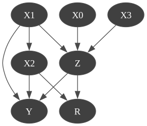

** Valdidation dataframe :

    X2  Y X0 X1  Z  R X3
0    1  1  0  1  0  1  0
1    0  1  1  1  0  2  0
2    0  1  0  1  1  2  1
3    1  1  1  0  1  1  0
4    0  0  1  1  0  4  0
..  .. .. .. .. .. .. ..
495  1  1  0  1  1  0  1
496  0  1  0  1  1  1  1
497  0  0  0  1  0  4  0
498  0  0  0  1  1  1  0
499  1  1  1  0  0  4  1

[500 rows x 7 columns]


** Log Likehood(validation): -3745.2452031757525

2-independence list (w.r.t. the class Y)

Given a model, it may be interesting to investigate the conditional independences encoded in the BN.

This function explores all the CI between 2 variables and computes the p-values w.r.t to a dataframe or a csv file.

## using the learning base
expl.independenceListForPairs(bn, data_path)

{('R', 'X0', ('X1', 'Z')): 0.7083382647903902,
 ('R', 'X1', ('X2', 'Z')): 0.4693848625409949,
 ('R', 'X3', ('X1', 'Z')): 0.4128522974536623,
 ('R', 'Y', ('X2', 'Z')): 0.8684231094674687,
 ('X0', 'X1', ()): 0.723302358657366,
 ('X0', 'X2', ()): 0.9801394906304377,
 ('X0', 'X3', ()): 0.7676868597218647,
 ('X0', 'Y', ('X1', 'Z')): 0.5816487109659612,
 ('X1', 'X3', ()): 0.5216508257424717,
 ('X2', 'X3', ()): 0.9837021981131505,
 ('X2', 'Z', ('X1',)): 0.6638491605436834,
 ('X3', 'Y', ('X1', 'Z')): 0.8774081450472305}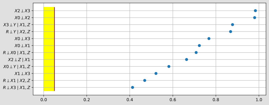

## or the validation dataframe
expl.independenceListForPairs(bn, validation)

{('R', 'X0', ('X1', 'Z')): 0.4170658306221731,
 ('R', 'X1', ('X2', 'Z')): 0.8772974188095352,
 ('R', 'X3', ('X1', 'Z')): 0.030295013169788092,
 ('R', 'Y', ('X2', 'Z')): 0.9762021037079481,
 ('X0', 'X1', ()): 0.3075057141178946,
 ('X0', 'X2', ()): 0.6811979505216854,
 ('X0', 'X3', ()): 0.18149463684324307,
 ('X0', 'Y', ('X1', 'Z')): 0.531775213130583,
 ('X1', 'X3', ()): 0.7676038150888187,
 ('X2', 'X3', ()): 0.243099916238547,
 ('X2', 'Z', ('X1',)): 0.22785672375855603,
 ('X3', 'Y', ('X1', 'Z')): 0.6803526498423738}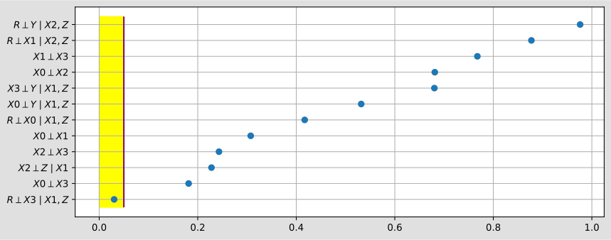

… with respect to a specific target.

expl.independenceListForPairs(bn, data_path, target="Y")

{('Y', 'R', ('X2', 'Z')): 0.8684231094674687,
 ('Y', 'X0', ('X1', 'Z')): 0.5816487109659612,
 ('Y', 'X3', ('X1', 'Z')): 0.8774081450472305}

3-SHAP values : explaining a Bayesian network as a classifier

print(expl.ConditionalShapValues.__doc__)

The ConditionalShapValues class computes the conditional Shapley values for a given target node in a Bayesian Network.

The ShapleyValues classes compute Shapley values in Bayesian networks. You must specify a target node. Each class (ConditionalShapValues, CausalShapValues, MarginalShapValues) takes the BN and target at construction; call .compute((dataframe, with_labels)) to obtain an Explanation object.

Compute Conditionnal in Bayesian Network

gumshap = expl.ConditionalShapValues(bn, "Y")

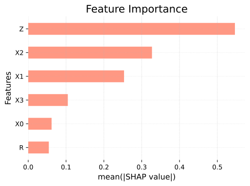
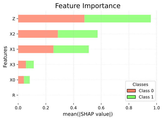
A dataset (as a pandas.DataFrame) must be provided. By default with_labels=True, meaning the data uses label strings instead of integer indices. To override, pass a tuple (df, with_labels) explicitly. The compute() method returns an Explanation object whose values and importances can be visualised with explnb.beeswarm() (distribution of shap values per variable) and explnb.bar() (variable importance ranking).

train = pd.read_csv(data_path).sample(frac=1.0)

t_start = time.time()
resultat = gumshap.compute(train)
explnb.beeswarm(resultat)
explnb.bar(resultat)
print(f"Run Time : {time.time() - t_start} sec")

Run Time : 1.009753942489624 sec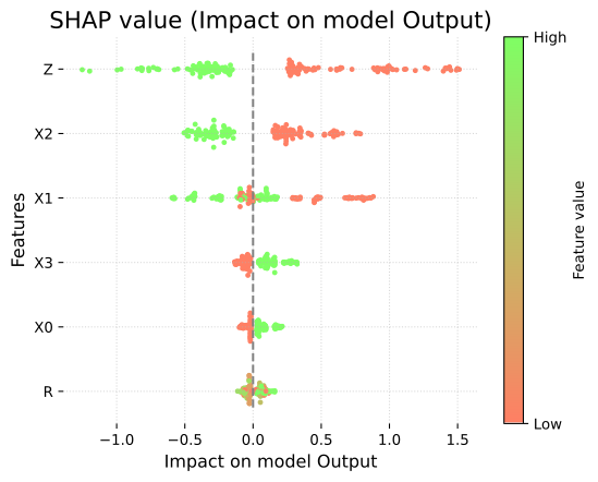

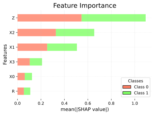
resultat = gumshap.compute(train)
explnb.bar(resultat)
explnb.bar(resultat, y=1)
print(f"Run Time : {time.time() - t_start} sec")

Run Time : 2.250892162322998 sec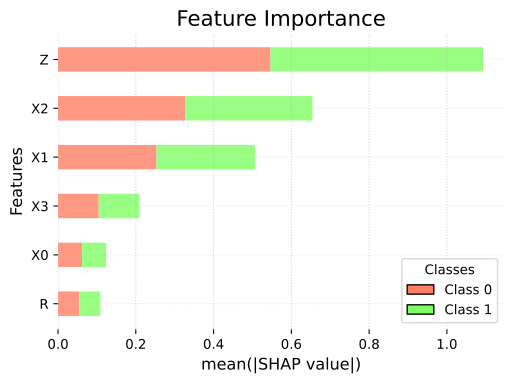

result = gumshap.compute(train)
explnb.beeswarm(result)
## result is an Explanation object with Shapley values for all nodes.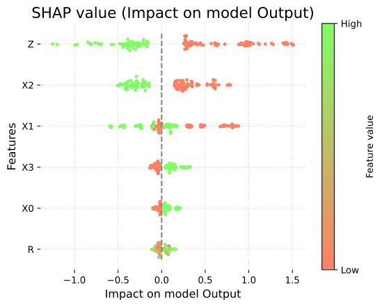

The result is an Explanation object (a MutableMapping). Its .importances attribute maps feature names to their average absolute Shapley value.

resultat = gumshap.compute(train)
print(f"Run Time : {time.time() - t_start} sec")

Run Time : 4.568569898605347 sec

Causal Shap Values

This method is similar to the previous one, except the formula of computation. It computes the causal shap value as described in the paper of Heskes Causal Shapley Values: Exploiting Causal Knowledge to Explain Individual Predictions of Complex Models .

t_start = time.time()
gumshap_causal = expl.CausalShapValues(bn, "Y", background=train)
causal = gumshap_causal.compute(train)
explnb.beeswarm(causal)
explnb.bar(causal)
print(f"Run Time : {time.time() - t_start} sec")

Run Time : 11.586209058761597 sec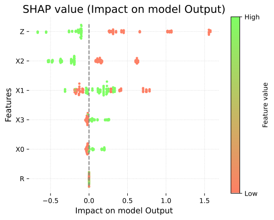

As you can see, since $R$ is not among the ‘causes’ of Y, its causal importance is null.

Marginal Shap Values

Similarly, one can also compute marginal Shap Value.

t_start = time.time()
gumshap_marginal = expl.MarginalShapValues(bn, "Y", background=train, sample_size=10)
marginal = gumshap_marginal.compute(train)
explnb.beeswarm(marginal)
explnb.bar(marginal)
print(f"Run Time : {time.time() - t_start} sec")

Run Time : 6.320684909820557 sec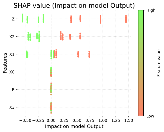

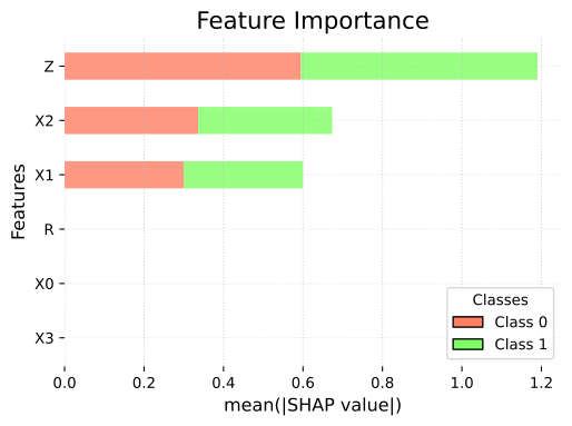
As you can see, since $R$, $X0$ and $X3$ are not in the Markov Blanket of $Y$, their marginal importances are null.

Saving the graph

Pass a filename argument to any plot function to save the figure to a file instead of displaying it:

import os

os.makedirs("out", exist_ok=True)

t_start = time.time()
causal2 = gumshap_causal.compute(train)
explnb.beeswarm(causal2, filename="out/beeswarm_causal.png")
explnb.bar(causal2, filename="out/bar_causal.pdf")
print(f"Run Time : {time.time() - t_start} sec")

Run Time : 11.816284894943237 sec

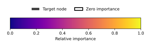
Visualizing SHAP values directly on a BN

This function returns a coloured graph that makes it easier to understand which variable is important and where it is located in the graph.

explnb.showShapValues(bn, causal, show_legend=True)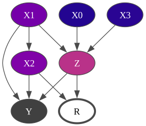

3-ShALL values : explaining the likelihood of a BN

While ShAP values explain why a BN classifies an observation as it does (contribution of each feature to $P(Y=y \mid x)$), ShALL values explain why the model assigns the likelihood it does to a complete observation (contribution of each feature to $\log P(x \mid \theta)$).

A ShALL explanation is always local: it decomposes the log-likelihood of one specific instance into per-feature contributions relative to a baseline. The natural visualisation is a waterfall chart.

We pick one specific observation from the validation set and explain its likelihood under the learned BN using ConditionalShallValues.

## Single instance from validation
instance = validation.iloc[[0]]
print(instance)

  X2  Y X0 X1  Z  R X3
0  1  1  0  1  0  1  0

gumshall = expl.ConditionalShallValues(bn, background=train)
shall_local = gumshall.compute(instance)
explnb.waterfall(shall_local)
print(shall_local)

Explanation(values={'X1': -0.21850608251964537, 'X2': -0.4070995156454551, 'Y': 0.012004341036384676, 'X3': 0.2492351342071131, 'Z': -0.0678958901371049, 'X0': 0.19679595096211683, 'R': 0.09311944650453617})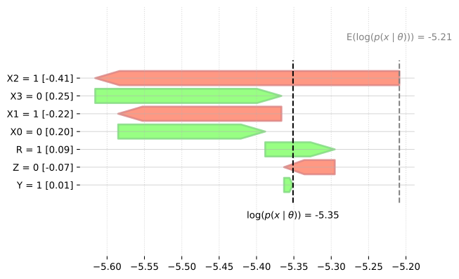

4- Visualizing information

Another view annotates the graph directly with information-theoretic quantities: each node is colored by its entropy (darker = lower, brighter = higher), and each arc thickness encodes the mutual information between its two endpoints (thicker = stronger statistical dependency). Pass show_legend=False to not display the scales.

expl.showInformation(bn)

expl.showInformation(bn, show_legend=False)