Kullback-Leibler for Bayesian networks

from pylab import *

import pyagrum and pyagrum.lib.notebook (for … notebooks :-) )

import pyagrum as gum
import pyagrum.lib.notebook as gnb

Create a first BN : bn

bn = gum.loadBN("res/asia.bgum")
## randomly re-generate parameters for every Conditional Probability Table
bn.generateCPTs()
bn

Create a second BN : bn2

bn2 = gum.loadBN("res/asia.bgum")
bn2.generateCPTs()
bn2

bn vs bn2 : different parameters

gnb.flow.row(bn.cpt(3), bn2.cpt(3), captions=["a CPT in bn", "same CPT in bn2 (with different parameters)"])

	positive_XraY
tuberculos_or_cancer	0	1
0	0.0305	0.9695
1	0.6024	0.3976

a CPT in bn

	positive_XraY
tuberculos_or_cancer	0	1
0	0.4978	0.5022
1	0.2117	0.7883

same CPT in bn2 (with different parameters)

Exact and (Gibbs) approximated KL-divergence

In order to compute KL-divergence, we just need to be sure that the 2 distributions are defined on the same domain (same variables, etc.)

Exact KL

g1 = gum.ExactBNdistance(bn, bn2)
print(g1.compute())

{'klPQ': 1.8158132012198116, 'errorPQ': 0, 'klQP': 2.2667305488649347, 'errorQP': 0, 'hellinger': 0.7776068053123616, 'bhattacharya': 0.3600179137754216, 'jensen-shannon': 0.3890583190550495}

If the models are not on the same domain :

bn_different_domain = gum.loadBN("res/alarm.bgum")

## g=gum.BruteForceKL(bn,bn_different_domain) # a KL-divergence between asia and alarm ... :(
#
## would cause
# ---------------------------------------------------------------------------
## OperationNotAllowed                       Traceback (most recent call last)
#
## OperationNotAllowed: this operation is not allowed : KL : the 2 BNs are not compatible (not the same vars : visit_to_Asia?)

Gibbs-approximated KL

g = gum.GibbsBNdistance(bn, bn2)
g.setVerbosity(True)
g.setMaxTime(120)
g.setBurnIn(5000)
g.setEpsilon(1e-7)
g.setPeriodSize(500)

print(g.compute())
print("Computed in {0} s".format(g.currentTime()))

{'klPQ': 1.8217614654099437, 'errorPQ': 0, 'klQP': 2.366125967018294, 'errorQP': 0, 'hellinger': 0.7834597610501289, 'bhattacharya': 0.3615380600381339, 'jensen-shannon': 0.3937662198925944}
Computed in 3.017523666 s

print("--")

print(g.messageApproximationScheme())
print("--")

print("Temps de calcul : {0}".format(g.currentTime()))
print("Nombre d'itérations : {0}".format(g.nbrIterations()))

--
stopped with epsilon=1e-07
--
Temps de calcul : 3.017523666
Nombre d'itérations : 682000

p = plot(g.history(), "g")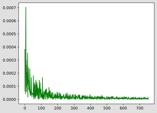

svg

Animation of Gibbs KL

Since it may be difficult to know what happens during approximation algorithm, pyAgrum allows to follow the iteration using animated matplotlib figure

g = gum.GibbsBNdistance(bn, bn2)
g.setMaxTime(60)
g.setBurnIn(500)
g.setEpsilon(1e-7)
g.setPeriodSize(5000)

gnb.animApproximationScheme(g)  # logarithmique scale for Y
g.compute()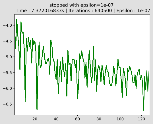

svg

{'klPQ': 1.81451760404998,
 'errorPQ': 0,
 'klQP': 2.258394235164226,
 'errorQP': 0,
 'hellinger': 0.7772834184516748,
 'bhattacharya': 0.35927611948575605,
 'jensen-shannon': 0.3889075347014891}

svg

Monte-Carlo-approximated KL

Unlike Gibbs sampling, MCBNDistance draws each sample independently (forward/topological sampling from P), with no Markov chain and therefore no burn-in.

mc = gum.MCBNDistance(bn, bn2)
mc.setVerbosity(True)
mc.setMaxTime(120)
mc.setEpsilon(1e-7)
mc.setPeriodSize(500)

print(mc.compute())
print("Computed in {0} s".format(mc.currentTime()))

{'klPQ': 1.8133039864732658, 'errorPQ': 0, 'klQP': 2.3498768717751863, 'errorQP': 0, 'hellinger': 0.7836402153493447, 'bhattacharya': 0.35779456438932733, 'jensen-shannon': 0.394466118361171}
Computed in 5.532348667 s

print("--")

print(mc.messageApproximationScheme())
print("--")

print("Temps de calcul : {0}".format(mc.currentTime()))
print("Nombre d'itérations : {0}".format(mc.nbrIterations()))

--
stopped with epsilon=1e-07
--
Temps de calcul : 5.532348667
Nombre d'itérations : 584000

p = plot(mc.history(), "b")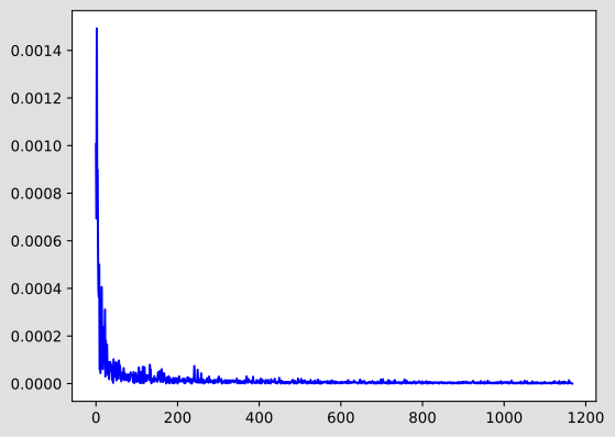

svg

Animation of Monte Carlo KL

Since it may be difficult to know what happens during approximation algorithm, pyAgrum allows to follow the iteration using animated matplotlib figure. As MCBNDistance draws independent samples at each iteration (no burn-in, no Markov chain), its convergence curve is usually smoother than Gibbs’.

mc = gum.MCBNDistance(bn, bn2)
mc.setMaxTime(60)
mc.setEpsilon(1e-7)
mc.setPeriodSize(5000)

gnb.animApproximationScheme(mc)  # logarithmique scale for Y
mc.compute()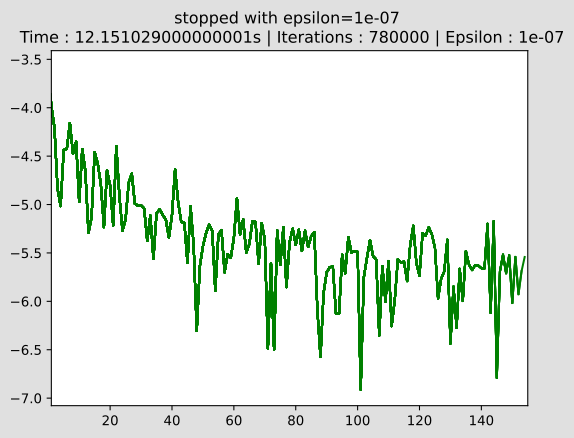

svg

{'klPQ': 1.8167797904168548,
 'errorPQ': 0,
 'klQP': 2.2366383000453633,
 'errorQP': 0,
 'hellinger': 0.7757017237555205,
 'bhattacharya': 0.3606491604142253,
 'jensen-shannon': 0.38744498890847345}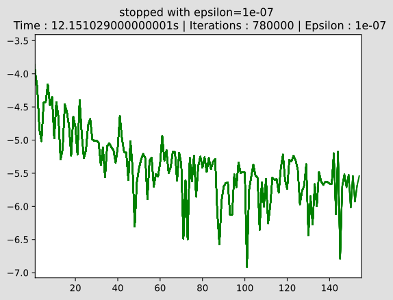

svg

Gibbs vs Monte Carlo : convergence towards the exact KL value

Since bn is small enough, we can compute the exact KL(P||Q) with ExactBNdistance and use it as ground truth. For a range of iteration budgets, we force both GibbsBNdistance and MCBNDistance to run exactly that many iterations (by disabling every other stopping criterion and setting periodSize to 1) and compare how fast their estimate of KL(P||Q) approaches the exact value.

exact = gum.ExactBNdistance(bn, bn2).compute()

iters = [100, 500, 1000, 5000, 10000, 50000]
nb_repetitions = 50

metrics = ["klPQ", "klQP", "hellinger", "bhattacharya", "jensen-shannon"]

gibbs_runs = {metric: [[] for _ in iters] for metric in metrics}
mc_runs = {metric: [[] for _ in iters] for metric in metrics}

for rep in range(nb_repetitions):
    for i, n in enumerate(iters):
        g = gum.GibbsBNdistance(bn, bn2)
        g.disableEpsilon()
        g.disableMinEpsilonRate()
        g.disableMaxTime()
        g.setPeriodSize(1)
        g.setBurnIn(50)
        g.setMaxIter(n)
        rg = g.compute()

        m = gum.MCBNDistance(bn, bn2)
        m.disableEpsilon()
        m.disableMinEpsilonRate()
        m.disableMaxTime()
        m.setPeriodSize(1)
        m.setMaxIter(n)
        rm = m.compute()

        for metric in metrics:
            gibbs_runs[metric][i].append(rg[metric])
            mc_runs[metric][i].append(rm[metric])

gibbs_mean = {metric: array([mean(vals) for vals in gibbs_runs[metric]]) for metric in metrics}
gibbs_sem = {metric: array([std(vals) for vals in gibbs_runs[metric]]) / sqrt(nb_repetitions) for metric in metrics}
mc_mean = {metric: array([mean(vals) for vals in mc_runs[metric]]) for metric in metrics}
mc_sem = {metric: array([std(vals) for vals in mc_runs[metric]]) / sqrt(nb_repetitions) for metric in metrics}

fig, axes = subplots(2, 3, figsize=(15, 8))
axes = axes.flatten()
for ax, metric in zip(axes, metrics):
    gm, gs = gibbs_mean[metric], gibbs_sem[metric]
    mm, ms = mc_mean[metric], mc_sem[metric]
    ax.plot(iters, gm, "o-", color="C0", label="Gibbs")
    ax.fill_between(iters, gm - gs, gm + gs, color="C0", alpha=0.3)
    ax.plot(iters, mm, "s-", color="C1", label="Monte Carlo")
    ax.fill_between(iters, mm - ms, mm + ms, color="C1", alpha=0.3)
    ax.axhline(y=exact[metric], color="k", linestyle="--", label="exact")
    ax.set_xscale("log")
    ax.set_xlabel("number of iterations")
    ax.set_ylabel(metric)
    ax.set_title(metric)
    ax.legend(fontsize=8)
axes[-1].axis("off")
fig.suptitle(f"Convergence of Gibbs and Monte Carlo estimates towards exact values\n(mean +/- std/sqrt({nb_repetitions}) over {nb_repetitions} repetitions)")
tight_layout()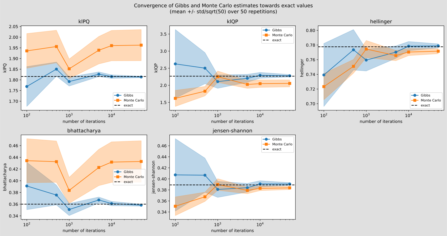

svg

In general, MCBNDistance converges better (faster, with a smaller variance) than GibbsBNdistance for a given number of iterations. This is expected: computing a distance between two BNs does not involve any observation (hard evidence) to account for during sampling, so there is no need for the Markov chain machinery (mixing, burn-in) that Gibbs sampling relies on to handle evidence. Drawing independent samples directly from P is both simpler and, here, more efficient.