Sensitivity analysis for Bayesian networks using credal networks

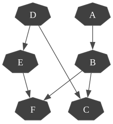
There are several sensitivity analysis frameworks for Bayesian networks. A fairly efficient method is certainly to use credal networks to do this analysis.

Creating a Bayesian network

import pyagrum.credal_net as gum
import pyagrum.lib.notebook as gnb

bn = gum.fastBN("A->B->C<-D->E->F<-B")
gnb.flow.row(bn, gnb.getInference(bn))

Building a credal network from a BN

It is easy to build a credal network from a Bayesian network by indicating the ‘noise’ on each parameter.

cr = gum.CredalNet(bn, bn)
gnb.show(cr)

cr.bnToCredal(1e-10, False, False)

cr.computeBinaryCPTMinMax()

print(cr)

A:Range([0,1])
<> : [[0.712502 , 0.287498] , [0.712498 , 0.287502]]

B:Range([0,1])

<A:0> : [[0.462944 , 0.537056] , [0.462787 , 0.537213]] <A:1> : [[0.675036 , 0.324964] , [0.675029 , 0.324971]]

C:Range([0,1])

<B:0|D:0> : [[0.296845 , 0.703155] , [0.294246 , 0.705754]] <B:1|D:0> : [[0.403277 , 0.596723] , [0.402866 , 0.597134]] <B:0|D:1> : [[0.320386 , 0.679614] , [0.31869 , 0.68131]] <B:1|D:1> : [[0.208129 , 0.791871] , [0.0823787 , 0.917621]]

D:Range([0,1])
<> : [[0.915245 , 0.0847542]]

E:Range([0,1])

<D:0> : [[0.376233 , 0.623767] , [0.375588 , 0.624412]] <D:1> : [[0.315478 , 0.684522] , [0.313626 , 0.686374]]

F:Range([0,1])

<E:0|B:0> : [[0.513989 , 0.486011] , [0.513918 , 0.486082]] <E:1|B:0> : [[0.909494 , 0.0905053]] <E:0|B:1> : [[0.349387 , 0.650613] , [0.348368 , 0.651632]] <E:1|B:1> : [[0.484391 , 0.515609] , [0.484279 , 0.515721]]

Testing difference hypothesis about the global precision on the parameters

We can therefore easily conduct a sensitivity analysis based on an assumption of error on all the parameters of the network.

def showNoisy(bn, beta):
  cr = gum.CredalNet(bn, bn)
  cr.bnToCredal(beta, False, False)
  cr.computeBinaryCPTMinMax()
  ielbp = gum.CNLoopyPropagation(cr)
  return gnb.getInference(cr, engine=ielbp)

for eps in [1, 1e-1, 1e-2, 1e-3, 1e-10]:
  gnb.flow.add(showNoisy(bn, eps), caption=f"noise={eps}")
gnb.flow.display()

noise=1

noise=0.1

noise=0.01

noise=0.001

noise=1e-10