Tensors and graphs

This notebook covers two related but independent low-level tools in pyAgrum : named Tensors (multi-dimensional arrays used to represent probability tables) and Graphs (the topological objects underlying every graphical model).

(Named) tensors

In pyAgrum>=2.0.0, Tensors (previously Potentials) represent multi-dimensionnal arrays with (discrete) random variables attached to each dimension. This mathematical object have tensorial operators w.r.t. to the variables attached.

import pyagrum as gum
import pyagrum.lib.notebook as gnb

va, vb, vc = [gum.LabelizedVariable(s, s, 2) for s in "abc"]

Tensor algebra

p1 = gum.Tensor(va, vb).fillWith([1, 2, 3, 4]).normalize()
p2 = gum.Tensor(vb, vc).fillWith([4, 5, 2, 3]).normalize()

gnb.flow.row(p1, p2, p1 + p2, captions=["p1", "p2", "p1+p2"])

	a
b	0	1
0	0.1000	0.2000
1	0.3000	0.4000

p1

	b
c	0	1
0	0.2857	0.3571
1	0.1429	0.2143

p2

		b
a	c	0	1
0	0	0.3857	0.6571
	1	0.2429	0.5143
1	0	0.4857	0.7571
	1	0.3429	0.6143

p1+p2

p3 = p1 + p2
p3 / p3.sumOut(["b"])

		c
b	a	0	1
0	0	0.3699	0.3208
	1	0.3908	0.3582
1	0	0.6301	0.6792
	1	0.6092	0.6418

p4 = gum.Tensor() + p3
gnb.flow.row(p3, p4, captions=["p3", "p4"])

		b
a	c	0	1
0	0	0.3857	0.6571
	1	0.2429	0.5143
1	0	0.4857	0.7571
	1	0.3429	0.6143

p3

		b
a	c	0	1
0	0	1.3857	1.6571
	1	1.2429	1.5143
1	0	1.4857	1.7571
	1	1.3429	1.6143

p4

Bayes’ theorem

bn = gum.fastBN("a->c;b->c", 3)
bn

In such a small bayes net, we can directly manipulate $P(a,b,c)$. For instance : $P(b|c)=\frac{\sum_{a} P(a,b,c)}{\sum_{a,b} P(a,b,c)}$

pABC = bn.cpt("a") * bn.cpt("b") * bn.cpt("c")
pBgivenC = pABC.sumOut(["a"]) / pABC.sumOut(["a", "b"])

pBgivenC.putFirst("b")  # in order to have b horizontally in the table

	b
c	0	1	2
0	0.2968	0.2256	0.4776
1	0.1267	0.0479	0.8254
2	0.3920	0.0619	0.5461

Joint, marginal probability, likelihood

Let’s compute the joint probability $P(A,B)$ from $P(A,B,C)$

pAC = pABC.sumOut(["b"])
print("pAC really is a probability : it sums to {}".format(pAC.sum()))
pAC

pAC really is a probability : it sums to 1.0

	a
c	0	1	2
0	0.1824	0.1198	0.0298
1	0.1998	0.1019	0.0366
2	0.2530	0.0231	0.0535

Computing $p(A)$

pAC.sumOut(["c"])

a
0	1	2
0.6353	0.2448	0.1199

Computing $p(A |C=1)$

It is easy to compute $p(A, C=1)$

pAC.extract({"c": 1})

a
0	1	2
0.1998	0.1019	0.0366

Moreover, we know that $P(C=1)=\sum_A P(A,C=1)$

pAC.extract({"c": 1}).sum()

0.3383032235186551

Now we can compute $p(A|C=1)=\frac{P(A,C=1)}{p(C=1)}$

pAC.extract({"c": 1}).normalize()

a
0	1	2
0.5907	0.3011	0.1082

Computing $P(A|C)$

$P(A|C)$ is represented by a matrix that verifies $p(A|C)=\frac{P(A,C)}{P(C}$

pAgivenC = (pAC / pAC.sumIn("c")).putFirst("a")
## putFirst("a") : to correctly show a cpt, the first variable have to bethe conditionned one
gnb.flow.row(pAgivenC, pAgivenC.extract({"c": 1}), captions=["$P(A|C)$", "$P(A|C=1)$"])

	a
c	0	1	2
0	0.5494	0.3609	0.0897
1	0.5907	0.3011	0.1082
2	0.7676	0.0702	0.1622

$P(A|C)$

a
0	1	2
0.5907	0.3011	0.1082

$P(A|C=1)$

Likelihood $P(A=2|C)$

A likelihood can also be found in this matrix.

pAgivenC.extract({"a": 2})

c
0	1	2
0.0897	0.1082	0.1622

A likelihood does not have to sum to 1. It is not relevant to normalize it.

pAgivenC.sumIn(["a"])

a
0	1	2
1.9077	0.7321	0.3601

Numpy interoperability

A Tensor’s content can be read as a numpy.ndarray (in the order of its variables) with toarray(), and built back from one with fillWith().

arr = pAC.toarray()
arr

array([[0.18243707, 0.11984106, 0.02980022],
       [0.19984102, 0.10185916, 0.03660304],
       [0.25302791, 0.02313105, 0.05345947]])

gum.Tensor(pAC).fillWith(arr)

	a
c	0	1	2
0	0.1824	0.1198	0.0298
1	0.1998	0.1019	0.0366
2	0.2530	0.0231	0.0535

tool on tensors : entropy of (probabilistic) tensor

%matplotlib inline
from pylab import *
import matplotlib.pyplot as plt
import numpy as np

p1 = gum.Tensor(va)
x = np.linspace(0, 1, 100)
plt.plot(x, [p1.fillWith([p, 1 - p]).entropy() for p in x])
plt.show()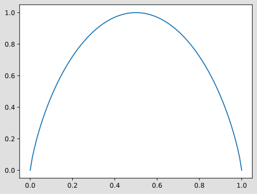

t = gum.LabelizedVariable("t", "t", 3)
p1 = gum.Tensor().add(t)


def entrop(bc):
  """
  bc is a list [a,b,c] close to a distribution
  (normalized just to be sure)
  """
  return p1.fillWith(bc).normalize().entropy()


import matplotlib.tri as tri

corners = np.array([[0, 0], [1, 0], [0.5, 0.75**0.5]])
triangle = tri.Triangulation(corners[:, 0], corners[:, 1])

## Mid-points of triangle sides opposite of each corner
midpoints = [(corners[(i + 1) % 3] + corners[(i + 2) % 3]) / 2.0 for i in range(3)]


def xy2bc(xy, tol=1.0e-3):
  """
  From 2D Cartesian coordinates to barycentric.
  """
  s = [(corners[i] - midpoints[i]).dot(xy - midpoints[i]) / 0.75 for i in range(3)]
  return np.clip(s, tol, 1.0 - tol)


def draw_entropy(nlevels=200, subdiv=6, **kwargs):
  refiner = tri.UniformTriRefiner(triangle)
  trimesh = refiner.refine_triangulation(subdiv=subdiv)
  pvals = [entrop(xy2bc(xy)) for xy in zip(trimesh.x, trimesh.y)]

  plt.tricontourf(trimesh, pvals, nlevels, **kwargs)
  plt.axis("equal")
  plt.ylim(0, 0.75**0.5)
  plt.axis("off")


draw_entropy()
plt.show()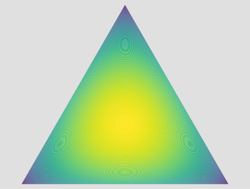

(Named) Graphs

aGrUM’s graph classes represent the topology of a graphical model, independently of variables or probability tables: pyagrum.DiGraph (arcs), pyagrum.UndiGraph (edges), pyagrum.MixedGraph (both), pyagrum.DAG (acyclic) and pyagrum.PDAG (partially directed, acyclic). Nodes are plain integers (NodeId); a name can optionally be attached to a node with setName.

g = gum.MixedGraph()
a, b, c = g.addNode(), g.addNode(), g.addNode()
g.setName(a, "A")
g.setName(b, "B")
g.setName(c, "C")
g.addArc(a, b)
g.addEdge(b, c)
gnb.show(g)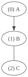

The fast syntax for graphs

Similarly to pyagrum.fastBN/pyagrum.fastMRF/pyagrum.fastID, graphs can be built from a compact dot-like description : '->' for a directed arc, '-' for an undirected edge, ';' to separate independent chains.

A single '-' (not '--') is used for edges on purpose : fastMRF already uses '--' to list the variables of a single factor (a clique), a different construct from a chain of pairwise edges. Writing 'A--B' in the functions below raises an error rather than being silently misread.

g1 = gum.fastDiGraph("A->B->C;B->E")
g2 = gum.fastUndiGraph("A-B-C")
g3 = gum.fastMixedGraph("A->B-C")
gnb.flow.row(g1, g2, g3, captions=["fastDiGraph", "fastUndiGraph", "fastMixedGraph"])

fastDiGraph

fastUndiGraph

fastMixedGraph

If every node token in the description is a plain (non-negative) integer, those integers are used directly as NodeIds instead of names :

sorted(gum.fastDiGraph("1->2->100").nodes())

[1, 2, 100]

fastDAG and fastPDAG enforce their own structural invariant while parsing, here fastDAG rejecting a directed cycle :

try:
  gum.fastDAG("A->B->C->A")
except gum.InvalidDirectedCycle as e:
  print(e)

[pyAgrum] Directed cycle detected: Add a directed cycle in a dag !

The convenience fastGraph entry point

pyagrum.fastGraph picks a graph type for you from a quick read of the description : arc-only descriptions try fastDAG first, falling back to fastDiGraph if that would create a directed cycle ; descriptions mixing arcs and edges try fastPDAG first, falling back to fastMixedGraph on the same condition ; edge-only descriptions build a fastUndiGraph.

g1 = gum.fastGraph("A->B->C;B->E")  # arcs only, no cycle -> DAG
g2 = gum.fastGraph("A->B-C")  # arcs and edges, no cycle -> PDAG
g3 = gum.fastGraph("A-B-C")  # edges only -> UndiGraph
gnb.flow.row(
  g1, g2, g3, captions=[f"fastGraph → {type(g1).__name__}", f"fastGraph → {type(g2).__name__}", f"fastGraph → {type(g3).__name__}"]
)

fastGraph → DAG

fastGraph → PDAG

fastGraph → UndiGraph

When the arcs alone would create a directed cycle, fastGraph falls back to the corresponding non-acyclic type instead of raising :

g4 = gum.fastGraph("A->B->C->A")  # a directed cycle -> DiGraph (not DAG)
g5 = gum.fastGraph("A->B->C->A;B-D")  # cycle + an edge -> MixedGraph (not PDAG)
gnb.flow.row(g4, g5, captions=[f"fastGraph → {type(g4).__name__}", f"fastGraph → {type(g5).__name__}"])

fastGraph → DiGraph

fastGraph → MixedGraph

Graph algorithms

Once built, graphs expose several structural algorithms.

dag = gum.fastDAG("Rain->WetGrass<-Sprinkler")
moral = dag.moralGraph()
gnb.flow.row(dag, moral, captions=["DAG", "moral graph"])

DAG

moral graph

DAG.dSeparation checks d-separation between (sets of) nodes given a conditioning set, without needing a full BayesNet :

rain, sprinkler, wetgrass = (dag.idFromName(n) for n in ["Rain", "Sprinkler", "WetGrass"])
print("Rain and Sprinkler d-separated (no conditioning) :", dag.dSeparation({rain}, {sprinkler}))
print("Rain and Sprinkler d-separated by WetGrass       :", dag.dSeparation({rain}, {sprinkler}, {wetgrass}))

Rain and Sprinkler d-separated (no conditioning) : True
Rain and Sprinkler d-separated by WetGrass       : False

Connected components and paths are available on undirected/mixed graphs :

g = gum.fastUndiGraph("A-B-C;D-E")
print("components  :", g.connectedComponentsList())
print("nb of comps :", g.connectedComponentsCount())

components  : {1: {3, 4}, 0: {0, 1, 2}}
nb of comps : 2

mg = gum.fastMixedGraph("A->B-C->D<-E<-F->B")
gnb.show(mg)
mg.mixedOrientedPath(mg.idFromName("A"), mg.idFromName("D"))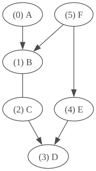

[0, 1, 2, 3]

mg.mixedOrientedPath(5,3) # from F to D

[5, 4, 3]