Dynamic Bayesian Networks
 |  |  |
Since pyAgrum>=3.2, dynamic Bayesian networks are no longer handled by the pure Python module pyagrum.lib.dynamicBN, which is now deprecated. They are handled by pyagrum.ktbn, a C++-backed module offering the same modeling capabilities with better performance and native inference on the k-TBN template.
import pyagrum as gumimport pyagrum.lib.notebook as gnbimport pyagrum.lib.dynamicBN as gdyn/var/folders/r1/pj4vdx_n4_d_xpsb04kzf97r0000gp/T/ipykernel_12561/461012950.py:3: FutureWarning: This module is deprecated since pyAgrum>=3.2. Please use the new c++ enhanced module : 'import pyagrum.ktbn' instead. import pyagrum.lib.dynamicBN as gdynThe table below illustrates how much better dBNs are now supported by this new C++ engine.
| Feature | Description |
|---|---|
KTBN construction | Build a k-TBN directly (add, addArc, generateCPTs) or from an existing KTBN-shaped BayesNet (KTBN.fromBN) |
| Naming convention | Temporal variables addressed as engine name "A[t]" or as the pair ("A", t) |
KTBNInference | Exact inference run directly on the template, without unrolling, for any horizon T |
| Learning | KTBNGenerator (random template generation), KTBNDatabaseGenerator (sample trajectories to CSV), KTBNAdaptiveLearner (learn structure and order k from data) |
| Engine | Implemented in C++, replacing the pure Python pyagrum.lib.dynamicBN |
import pyagrum.ktbn as gum # gum+ktbnBuilding a 2TBN
Section titled “Building a 2TBN”A 2TBN is simply a k-TBN with . Following the pyagrum.ktbn naming convention, a temporal variable named has one instance per time slice of the template, addressed either as the engine name A[0]/A[1] or as the pair ("A", 0)/("A", 1). Slice 0 is the initial slice and slice 1 — the last of the template — is the (time-homogeneous) transition kernel, reused for every once unrolled.
However, following the old dynamicBN convention, it is possible to declare a KTBN using a BN with variables name ending with the timeslice (A0/A1/etc.). Once the ktbn is built, the true names of the variable is A[0]/A[1]/etc.
## same structure as gum.fastBN("d0[3]->ct<-at<-a0->b0->bt<-a0->dt[3]<-d0<-c0->ct;c0->at", 6)## but built directly with pyagrum.ktbn : there is (yet) no fast-string constructor for a KTBN## twodbn = gum.KTBN(2)## for name in ["a", "b", "c"]:#  twodbn.add(gum.fastVariable(f"{name}[6]"))## twodbn.add(gum.fastVariable("d[3]"))
## for base1, s1, base2, s2 in [# ("a", 0, "a", 1),# ("a", 0, "b", 0),# ("a", 0, "b", 1),# ("a", 0, "d", 1),# ("c", 0, "d", 0),# ("c", 0, "c", 1),# ("c", 0, "a", 1),# ("d", 0, "c", 1),# ("d", 0, "d", 1),# ("b", 0, "b", 1),# ("a", 1, "c", 1),# ]:# twodbn.addArc(base1, s1, base2, s2)## twodbn.generateCPTs()bn = gum.fastBN("d0[3]->c1<-a1<-a0->b0->b1<-a0->d1[3]<-d0<-c0->c1;c0->a1", 6)bnUnlike a plain pyagrum.BayesNet relying on a naming convention to be recognized as a 2TBN, KTBN knows about its two time slices.
twodbn = gum.KTBN.fromBN(bn)print("k =", twodbn.k(), " / arcs =", twodbn.sizeArcs())gnb.show(twodbn)k = 2 / arcs = 11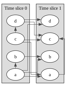
unrolling 2TBN
Section titled “unrolling 2TBN”A k-TBN is ‘unrolled’ using unroll(T), T being the number of time slices. For the couple , in the template, the unrolled BN will include .
T = 5
bn = twodbn.unroll(T)gnb.showBN(bn, size="10")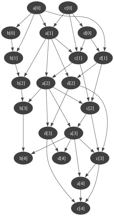
We can infer on bn just as on a normal BN. Following the k-TBN engine-name convention, the variables in the unrolled BN are named base[i] where i is the number of their time slice.
gnb.flow.clear()for i in range(T): gnb.flow.add(gnb.getPosterior(bn, target=f"d[{i}]", evs={}), f"$P(d[{i}])$")gnb.flow.display()


dynamic inference : following variables
Section titled “dynamic inference : following variables”gum.KTBNInference runs exact inference directly on the k-TBN template — without ever unrolling it — for any horizon T. Observations can be placed at any absolute time slice using the engine-name convention (e.g. "a[9]"); posteriors(base) then returns the whole series for , which we stack-plot below, just like gdyn.plotFollow used to.
import matplotlib.pyplot as plt
plt.rcParams["figure.figsize"] = (10, 2)
gnb.plotFollowKTBN(  twodbn,  ["a", "b", "c", "d"],  T=51,  observations={"a[9]": 2, "a[30]": 0, "c[14]": 0, "b[40]": 0, "c[50]": 3},)
nsDBN (Non-Stationnary Dynamic Bayesian network)
Section titled “nsDBN (Non-Stationnary Dynamic Bayesian network)”The pyagrum.ktbn module does not (yet) model non-stationary dBNs as such : a KTBN always assumes the same k-TBN template is reused for every time slice. In the meantime, a non-stationary dBN can still be simulated by unrolling a k-TBN into a plain pyagrum.BayesNet with unroll(T), and then editing that unrolled network directly — changing arcs and CPTs for the time slices where the dynamics differ, as shown below.
T = 15
bn = twodbn.unroll(T)gnb.showBN(bn)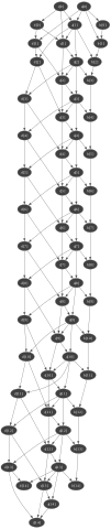
Non-stationary dBN allows to express that the dBN does not follow the same 2TBN during all steps. gum.unroll() returns a classical pyagrum.BayesNet, which can then be changed as you want, exactly as with an unrolled 2TBN before.
##### new P(c[t]|c[t-1])pot = gum.Tensor().add(twodbn.variable("c", 1)).add(twodbn.variable("c", 0))pot.fillWith([1, 0, 0, 0.1] * 9).normalizeAsCPT() # 36 valeurs normalized as CPT|
|
|
|
|
|
| |
|---|---|---|---|---|---|---|
| 0.4762 | 0.0000 | 0.0000 | 0.0476 | 0.4762 | 0.0000 | |
| 0.0000 | 0.0833 | 0.8333 | 0.0000 | 0.0000 | 0.0833 | |
| 0.4762 | 0.0000 | 0.0000 | 0.0476 | 0.4762 | 0.0000 | |
| 0.0000 | 0.0833 | 0.8333 | 0.0000 | 0.0000 | 0.0833 | |
| 0.4762 | 0.0000 | 0.0000 | 0.0476 | 0.4762 | 0.0000 | |
| 0.0000 | 0.0833 | 0.8333 | 0.0000 | 0.0000 | 0.0833 | |
## from steps 5 to 10, C_t only depends on C_{t-1} and follows this new CPTfor i in range(5, 11):  bn.eraseArc(f"d[{i - 1}]", f"c[{i}]")  bn.eraseArc(f"a[{i}]", f"c[{i}]")  bn.cpt(f"c[{i}]").fillWith(pot, ["c[1]", "c[0]"])  # c[1] in pot <- node itself, c[0] in pot <- parent
gnb.showBN(bn, size="14")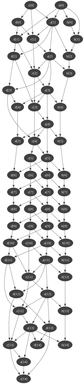
Since a non-stationary unrolled BN no longer matches the k-TBN template, KTBNInference no longer applies here : we fall back to a plain LazyPropagation over the unrolled BN, exactly what gdyn.plotFollowUnrolled used to do — reimplemented locally since pyagrum.lib.dynamicBN is retired.
import numpy as npfrom matplotlib.patches import Rectangle

def plotFollowUnrolled(lovars, bn, T, evs):  ie = gum.LazyPropagation(bn)  ie.setEvidence(evs)  ie.makeInference()
  x = np.arange(T)  for var in lovars:    v0 = bn.variableFromName(f"{var}[0]")    lpots = []    for i in range(v0.domainSize()):      serie = [ie.posterior(bn.idFromName(f"{var}[{t}]"))[i] for t in range(T)]      lpots.append(serie)
    _, ax = plt.subplots()    plt.xlim(left=0, right=T - 1)    plt.ylim(top=1, bottom=0)    ax.xaxis.grid()    plt.title(f"Following variable {var}", fontsize=20)    plt.xlabel("time")
    stack = ax.stackplot(x, lpots)    proxy_rects = [Rectangle((0, 0), 1, 1, fc=pc.get_facecolor()[0]) for pc in stack]    labels = [v0.label(i) for i in range(v0.domainSize())]    plt.legend(proxy_rects, labels, loc="center left", bbox_to_anchor=(1, 0.5), ncol=1, fancybox=True, shadow=True)    plt.show()

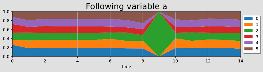
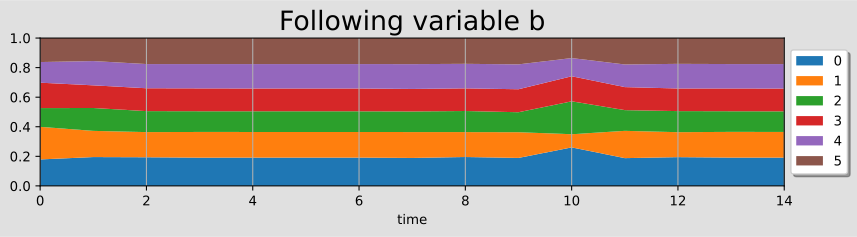
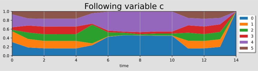
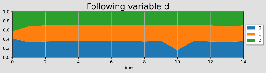
plt.rcParams["figure.figsize"] = (10, 2)plotFollowUnrolled(["a", "b", "c", "d"], bn, T=15, evs={"a[9]": 2, "c[14]": 0})